Sage Journals: Discover world-class research

Abstract

At present, the commonly used task scheduling methods of automated guided vehicle do not fully consider the influence of power consumption, the workshop environment, and other factors, resulting in the disparity between scheduling methods and practical applications. This article contributes to filling this gap by modifying the model and algorithm that can meet the real-time application in the factory. First, a scheduling model is established according to both the number of depots and the automated guided vehicle’s battery consumption, so that the result of task allocation is more reasonable. Then, according to the area, distribution, shape characteristics of obstacles, and the number of depots contained in the environment, this article derives a new coefficient which is constructed as the weighted value of the distance between workstations to improve the robustness of the model. Finally, the modified genetic algorithm is used to obtain the scheduling results. The simulation results show the effectiveness and the rationality of the proposed method.

Keywords

Automated guided vehicles scheduling map complexity coefficient GA

Introduction

Automated guided vehicles (AGVs) are driverless mobile vehicles that enable the minimization of human–labor interventions on tedious, time-consuming, and sometimes hazardous jobs.¹ With the development of the trackless AGV, many of today’s logistics and manufacturing processes rely on the use of multiple automated guided vehicle (multi-AGV) systems.² In order to make multi-AGV systems fully perform, the key issues to be solved involve task scheduling and path planning for all AGVs.

Scheduling is concerned with the allocation of limited resources to tasks over time and is a decision-making process that links the operations, time, cost, and overall objectives of the company.³ Especially in the flexible manufacturing system(FMS), the FMS performance increases by better coordination and scheduling of its components like AGV.^4
–6 However, the scheduling problem is an Non-deterministic Polynomial (NP)-hard problem.⁷ Most of the existing studies use powerful heuristic algorithms^8
–10 or Petri net methods¹¹ to solve these problems. Besides, the multi-AGV scheduling problem is always presented by an undirected graph and its solution is obtained by searching this graph for an optimum route satisfying the related constraints.¹² Most of the versions of the problem assume that each AGV runs at a fixed route between the workstations. However, in the actual workshop environment, in order to avoid obstacles, the AGV’s route is more complicated, which leads these versions to have poor applications.

Furthermore, after assigning tasks to all AGVs, each AGV needs path planning to complete the delivery task. It is true that the path planning aims to find a collision-free path from a start location to a target location while optimizing one or more objectives like path length, smoothness, and safety at a time.¹³ However, path planning and scheduling problems are usually studied separately. This is because integrated scheduling and path planning form a very challenging NP optimization problem.¹⁴ In recent years, Xidias and his coworkers^12,15,16 utilized the concept of Bump-surfaces¹⁷ to solve this integration problem. There is a drawback which shows the computational time will increase significantly when the number of workstation exceeds 15, although these researches perform a global search of the solution space in order to ensure an optimal scheduling and path planning for the set of AGVs.

In practical application, manufacturing enterprises are facing fierce market competition and an urgent need to improve efficiency. Therefore, whenever the order is issued, the scheduling result should be allocated quickly. To meet the real-time requirements, this article adopts the method, which firstly calculates the scheduling results and then plans the path. Compared with the integrated approach, this method is not able to increase the time complexity of the algorithm, but it lacks application in different environments. To address the above concerns, this article derives a map complexity coefficient which is regarded as the weighted value of the distance between workstations according to the given 2-D environment. In addition, the battery charge of the AGV is also an important constraint for task allocation. If proper battery management is used in the multi-AGV system, the system cost can be reduced, and the system efficiency can be improved.¹⁸ However, many studies do not consider the AGV’s battery charge and that leads to impracticable scheduling models.¹⁹ Therefore, the scheduling model of this article considers this constraint and performs the task allocation according to the remaining battery charge of each AGV. Then, a modified GA is proposed to calculate this scheduling model. In the path planning stage, a prioritized planning algorithm²⁰ is introduced to assign priorities according to the battery charge (the lower the charge is, the higher the priority is). The AGV is run according to the avoidance rules of the prioritized planning algorithm.

The novelties of this article lie in the following:

Unlike the traditional AGV scheduling model, this article optimizes the power consumption of the AGV as a target, considering whether the remaining battery charge of the AGV meets the scheduling task requirements.

By proposing the map complexity coefficient to improve the scheduling model, the scheduling results are more suitable for actual factory applications.

In view of the two factory environments of multi-depot and single depot, genetic algorithms are modified to obtain the optimal solutions of the two models.

The rest of the article is organized as follows. The problem statement and mathematical formulation are described in the second section; the third section illustrates the modifications of the genetic algorithm; the fourth section presents briefly the path planning algorithm; the experimental results are given in the fifth section; the sixth section concludes the article.

Problem statement and mathematical formulation

Facility layout

A workshop equipped with multi-AGV scheduling system should include N workstations, M AGVs (N > M), and some obstacles (shelves, machine tools, walls, etc.). This article considers the situation of AGVs going to and from a single depot and multiple depots. As shown in Figure 1, case one is a 2-D environment that contains only one depot. Case two is a 2-D environment with multiple depots.

Figure 1.

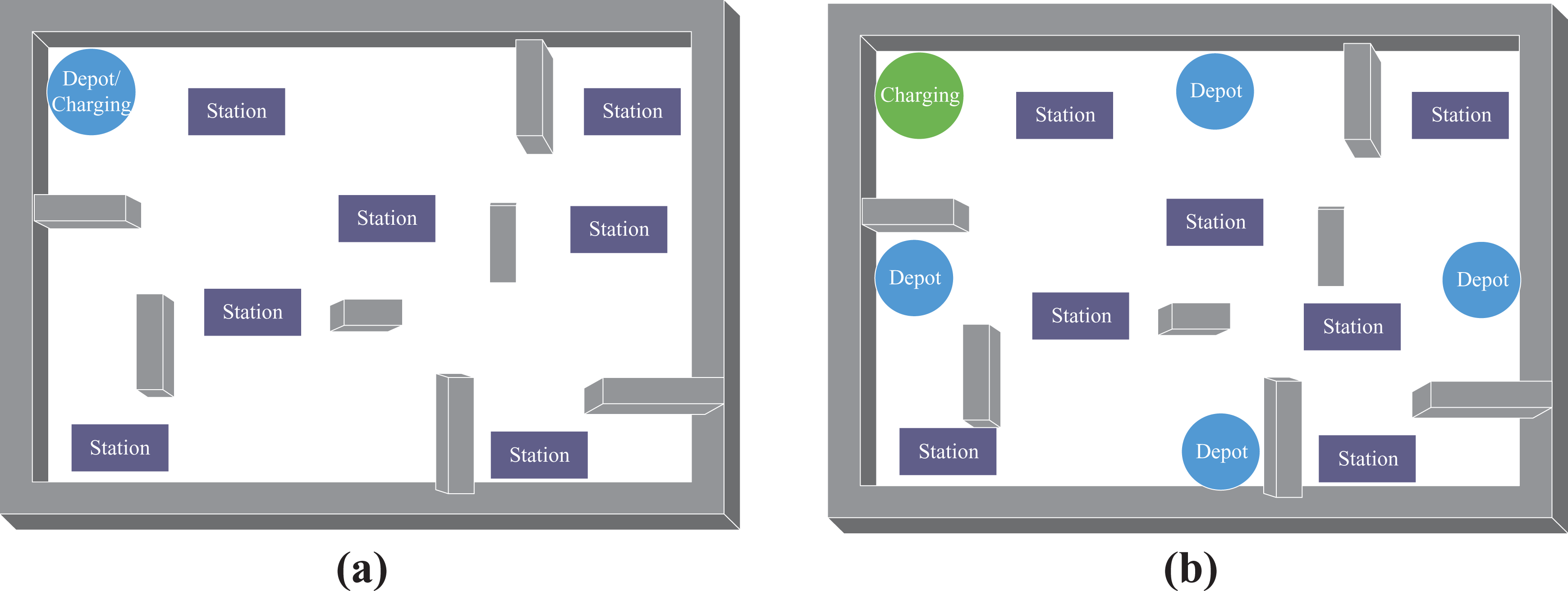
2-D workshop environment diagrams: (a) case 1 and (b) case 2.

In Figure 1, the gray areas are obstacles, and the blue areas are the depots (AGV starting point), the green area is the battery charging area of AGV (the top left corner of case one is both the depot and the charging area), and the purple areas are the workstations. The assumptions are as follows:

– Each AGV has to start from its starting depot and return to the same depot after completing the task.

– When the delivery task is finished, AGV will go to the charging area, if the power is below a threshold.

– Only one AGV passes through each workstation (except the starting point).

– The number of AGVs (or depots) is less than the number of workstations.

– For the workshop with multiple depots, each depot only sends one AGV at a task.

Model derivation

Based on the existing mathematical model,²¹ the following improvements are made: (a) constructing a map complexity coefficient as a weighted value of the distance between workstations; (b) the objective function gives priority to the solutions with the minimum total power consumption of all AGVs and then selects the scheme that minimizes the makespan, (c) considering the power consumption of AGV. The improvement model is as follows:

1. Notations

M	total number of AGVs
N	total number of workstations
d	total number of depots in an environment
i, j	indexes for two workstations on the ends of an arc, $i = 0, 1, 2, ..., N; j = 0, 1, 2, ..., N$
k	index for AGVs numbers, $k = 1, 2, ..., M$
l	index for the workstations requires AGVs to delivery, $l = 1, 2, ..., L_{k}; 0 < L_{k} < N$
$R_{i j}$	arc between two workstations i and j
$C_{i j}$	length of the corresponding arc segment $R_{i j}$
γ	power consumption coefficient corresponding to the path
ε	map complexity coefficient
$B_{k}$	power consumed by the k-th AGV
$L B_{k}$	maximum allowable power consumption of AGV in the current task
$p_{k}$	starting point of the k-th AGV
$i n i B_{k}$	initial battery charge of k-th AGV
$T_{k}$	value of the charge threshold of k-th AGV
S_i	total area of the obstacles
S	total area of the workshop
σ	standard deviation of the areas of the evenly divided map
μ	total number of consecutive obstacles of a map

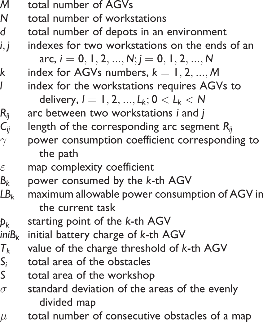
2. Variables

X_{i j k} = {\begin{cases} 1, the k -th AGV passes the arc R_{i j} \\ 0, otherwise \end{cases}

Y_{k i} = {\begin{cases} 1, the k -th AGV goes to the i -th station \\ 0, otherwise \end{cases}

B_{k} = (\sum_{i = 0}^{L_{k}} \sum_{j = 0}^{L_{k}} γ C_{i j} X_{i j}) ε

3. Objective function

J = min (\sum_{k = 1}^{M} B_{k}) \cap min (max (B_{k}))

4. Requirements

\sum_{k = 1}^{M} Y_{k i} = {\begin{cases} M, i = 0 \\ 1, i = 1, ..., L_{k} \end{cases}

\sum_{i = 0}^{L_{k}} X_{i j k} = Y_{k j}, j = 0, ..., L_{k}, k = 1, ..., M

\sum_{j = 0}^{L_{k}} X_{i j k} = Y_{i}, i = 0, ..., L_{k}, k = 1, ..., M

{\begin{cases} B_{k} \leq L B_{k}, allocated successfully \\ otherwise, reassignment \end{cases}

where ε is a map complexity coefficient, which is discussed in section “The derivation of the map complexity coefficient.” γ is a power consumption coefficient corresponding to the path. According to the type of batteries used, charging methods, charge rate, application, manufacturer, and assignments the vehicles perform, AGV battery-run-time and battery-charging-time can be defined. In order to adapt to any kind of battery, charging method, a coefficient $γ_{t}$ for transforming energy consumption to time was defined.¹⁹ Ignoring the amount of power consumed by the AGV when it stops at the station, the battery level of AGV can be regarded as gradual consumption in the course of driving. When AGV travels at a uniform speed v, the relationship between the γ and $γ_{t}$ is $γ = γ_{t} \times v$ .

In the above model, equations (1), (2), (5), (6), and (7) are adopted from the existing model.²¹ The scheduling problem is a combinatorial optimization problem, which has many feasible solutions. In this model, it gives priority to the solutions with the minimum total power consumption of all AGVs and then selects the scheme that minimizes the makespan, so the multi-objective optimization function is used. Since the amount of power consumption is related to the run-time of the AGV, minimizing the makespan is equivalent to minimizing the maximum power consumption of the AGV. For example, there are three AGV-assigned tasks. Assuming that both schemes satisfy 60% of the total power consumption, that is, the three AGV power consumptions of scheme one are 16%, 15%, and 29%, respectively. The second scheme is 17%, 18%, 25%. Because the maximum power consumption of AGV in the second scheme is 25%, which is lower than 29% in scheme one, the second option is the final result.

Requirement (5) specifies that each AGV starts from the starting depot “0,” all workstations can only be accessed once by an AGV. Requirement (6) shows that any arc starts from the starting depot. Requirement (7) implies that any arc ends with the starting depot. Requirement (8) make sure the assigned AGV has enough battery charge to do the job.

However, the above formulas apply to case 1 of Figure 1. For multiple depots, the following improvements should be made to constraints (5) to (7).

\sum_{k = 1}^{M} Y_{k i} = {\begin{cases} M, i = p_{k} \\ 1, i =1, ... L_{k} \end{cases}

\sum_{i = p k}^{L_{k}} X_{i j k} = Y_{k j}, j = p_{k}, ..., L_{k}, k = 1, ..., M

{\begin{cases} i f i n i B_{k} - B_{k} \leq T_{k} \\ \sum_{j = 0}^{L_{k}} X_{i j k} = Y_{k i}, i = 0, ..., L_{k}, k = 1, ..., M \\ i f i n i B_{k} - B_{k} > T_{k} \\ \sum_{j = p_{k}}^{L_{K}} X_{i j k} = Y_{k i}, i = p_{k}, ..., L_{k}, k = 1, ..., M \end{cases}

wherein requirements (9) and (10) show that each AGV starts from its own depot. After the delivery task is completed, requirement (11) represents that if AGV battery power is low (below $T_{k}$ ), the AGV will go to the charging area on its own, otherwise it will return to its starting depot.

The derivation of the map complexity coefficient

In most of the existing scheduling model, there is no obstacle in the workshop. However, when there are obstacles (static or dynamic) in the environment, the actual routes are complicated. In order to calculate more accurately during the scheduling, it is necessary to construct the ε.

In the actual workshop environment, most of the obstacles are some regular objects, such as shelves, machine tools, boxes, and so on. The area, distribution, and shape characteristics of these objects in the workshop are the important factors of the workshop environment complexity. This article is based on these factors to derive the map complexity coefficient. Therefore, ε should satisfy the condition of $ε \geq 1$ , when $ε =1$ , there is no obstacle in the environment.

The first factor to affect the AGVs’ route is the area of obstacles. As shown in Figure 2, the different area of the obstacles, the AGV driving route will be affected.

Figure 2.

The impact of the area of an obstacle: (a) small area and (b) large area of the obstacle.

Therefore, the following formula can be derived according to the area proportion of the obstacles in the environment.

ε =1+ \frac{S_{i}}{S}

where $S_{i}$ is the total area of the obstacles, and S is the total area of the workshop.

Although the area of obstacles is an important parameter, the difference of obstacle distribution in the workshop will also have a great impact. As shown in Figure 3, the area proportion of the obstacles in the map is equal, but the routes of AGV are different.

Figure 3.

The impact of obstacle distribution: (a) dispersed distribution of obstacles and (b) concentrated distribution of obstacles.

From Figure 3 we can see that although the area of obstacles is the same, the result of equation (12) cannot adapt to the two situations at the same time. To address this problem, the map can be evenly divided into lots of small pieces to calculate the area of obstacles in each small piece and then calculate the standard deviation σ of these areas, which can reflect the obstacle distribution degree (to improve the calculation accuracy, map division number should not be too small). As shown in Figure 4, the map is equally divided into 25 blocks using a series of equidistant lines (blue straight lines)

Figure 4.

The method of divide.

Therefore, equation (12) is changed to

ε =1+ (\frac{S_{i}}{S} \times e^{\frac{1}{1 + σ}})

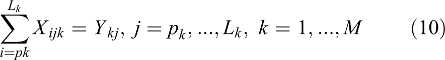
where e is a natural constant. $e^{\frac{1}{1 + σ}}$ represents the effect of the distribution of obstacles. For the case of the same total obstacles area, if the obstacles are concentrated in a certain region of the environment (σ is larger), then the region will have a major impact on the run of AGV, but the overall impact on the whole environment is not large, at this time, the result of (13) will be smaller. On the other hand, if the obstacles are more evenly distributed in all regions of the map (σ is a smaller value), the comprehensive impact of the whole environment will be large, the result of (13) will be a larger value.

In addition, the shape characteristics of obstacles cannot be ignored. Because some kinds of obstacle reduce the passages of AGV, this situation will still increase the detour degree of AGV. Figure 5 provides a clearer illustration of this problem.

Figure 5.

The impact of the shape characteristics of the obstacle: (a) discontinuous obstacle and (b) continuous obstacle.

As shown in Figure 5, for longer or wider obstacles, some passages in the middle, it can facilitate the driving of AGV. If there are fewer passages, the detour degree will increase. In this case, we define these obstacles as follows: if an obstacle is in the driving area of AGV, and the dimension of the obstacle exceeds a certain length in the direction of X-axis or Y-axis, it cannot provide a driving passage for the AGV, then it is regarded as a “continuous obstacle.” For accurate calculation, this article stipulates that if the obstacle size exceeds one-third of the length of the workshop in either the X-axis or the Y-axis, this obstacle is one continuous obstacle. If it exceeds two-thirds, then this obstacle will be regarded as two continuous obstacles.

Formula (13) is updated to

ε =1+ (\frac{S_{i}}{S} \times e^{\frac{1}{1 + σ}} \times ln (μ + e))

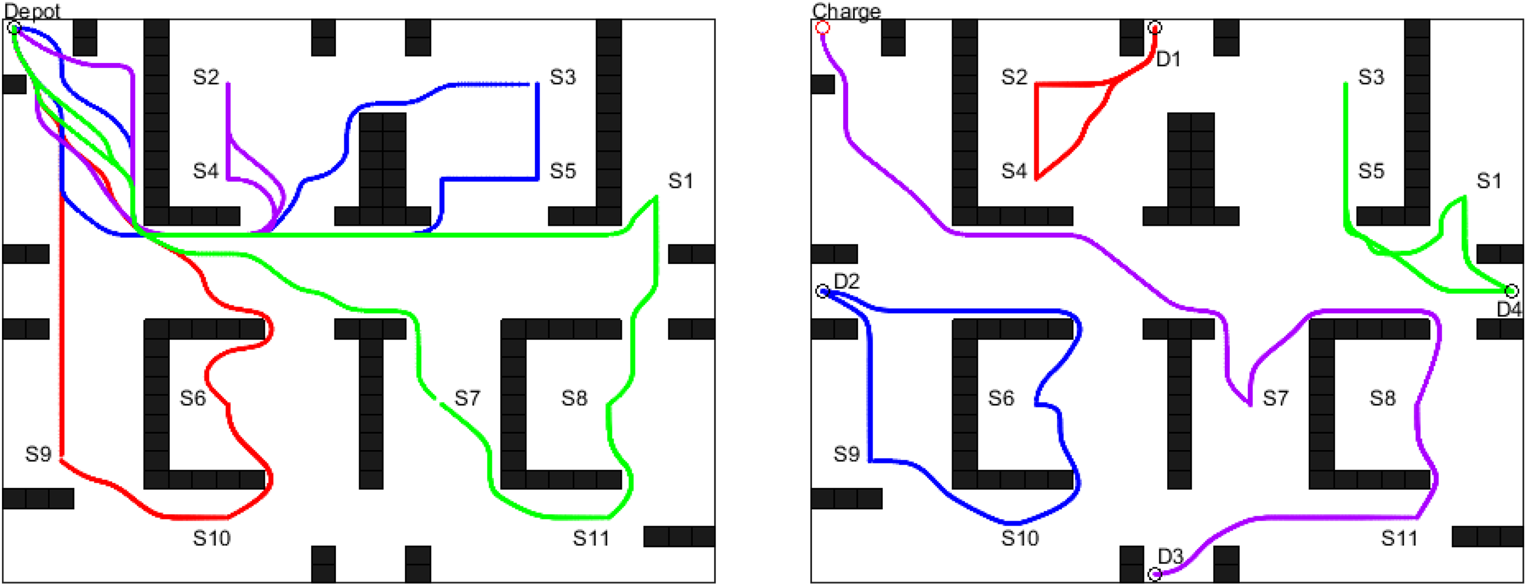
where μ is the number of continuous obstacles. $ln (μ + e)$ is the impact of continuous obstacles. In the absence of such obstacles ( $μ =0$ ), then $ln (μ + e)$ takes a value of 1. When this kind of obstacles is present ( $μ > 0$ ), it increases the value of ε.

The above content has analyzed the impact of obstacles in the environment map in detail, but some workshop environments only arrange one depot as the starting point of AGV, while others arrange multiple depots. Figure 6 shows the situations of AGV travelling to and from the same starting point and multiple starting points. The green lines and the red lines, respectively, represent the routes of two different AGVs. When the environment contains multiple depots, in order to save the AGV’s battery power, each AGV preferentially selects a station closer to it for material distribution.

Figure 6.

The impact of the number of depots: (a) the environment with one depot and (b) the environment with one depots.

In order to make formula (14) adapt to the above two situations, the following improvements are made to formula (14)

ε =1+ [\frac{S_{i}}{S} \times e^{\frac{1}{1 + σ}} \times ln (μ + e) \times \frac{N - (d - 1)}{N}] (d = 1,2, ..., N)

In formula (15), when the number of depots (d) is 1, the result is equal to formula (14). As the number of depots increases, the value of the equation will be reduced gradually, so formula (15) is a more general form of formula (14). Finally, we define equation (15) as a calculation formula for map complexity.

The modified genetic algorithm

In this article, the GA is used to calculate the model. A typical genetic algorithm includes genetic coding, selection action, crossover operation, and mutation operation. Considering the constraint of AGVs’ battery consumption, this article has made some improvements in GA. First of all, for the workshop environment with a single depot, the new constraint is to judge whether the decoded scheduling results match to meet the battery power of each AGV. Therefore, we have added an operation to judge the obtained result (operation 1):

Step 1. Input: the maximum allowable power consumption of each AGV ( $L B_{1}, L B_{2}, ..., L B_{k}$ ).

Step 2. Decode: the current chromosomal corresponding results ( $B_{1}, B_{2}, ..., B_{k}$ ).

Step 3. Sort the results of steps 1 and 2 in ascending order, respectively: $M M =sort ([L B_{1}, L B_{2}, ..., L B_{k}])$ , $N N =sort ([B_{1}, B_{2}, ..., B_{k}])$ .

Step 4. If $N N_{k} \leq M M_{k}, forall k = 1, 2, ..., M$ , accept the new solutions. Otherwise, abandon the new solutions.

From the above steps, the process of energy consumption judgement is obtained. After adding this process to the genetic algorithm, the flowchart as shown in Figure 7(a).

Figure 7.

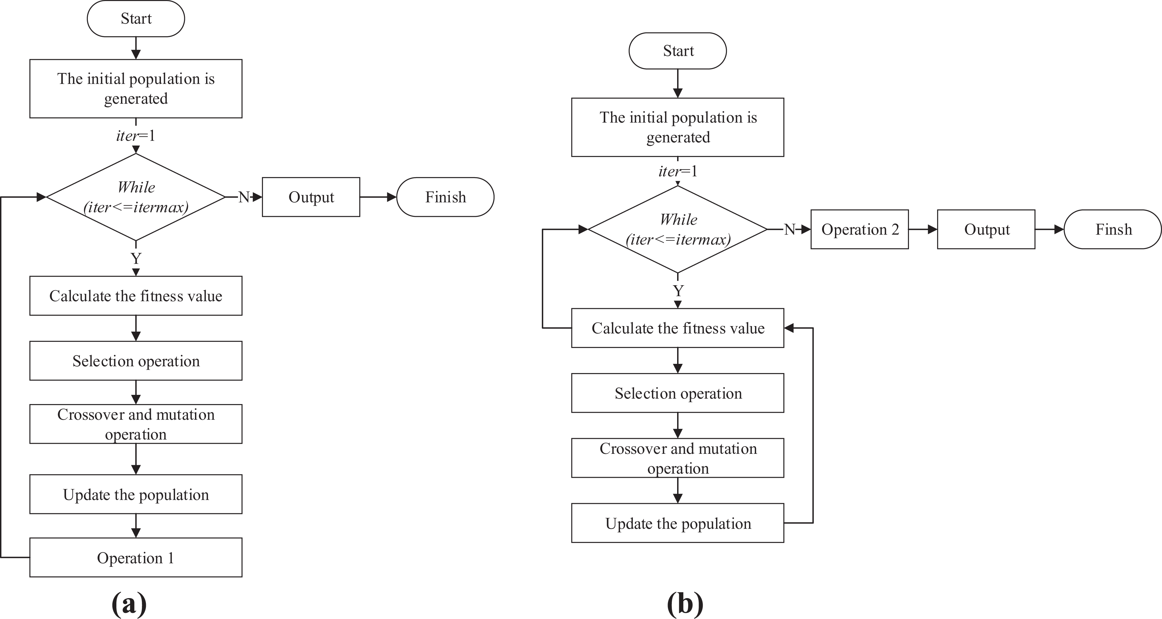
Flowcharts of GA. GA: genetic algorithm.

Then, for the workshop with multiple depots, after the task is completed, each AGV should return to their own depots when the electricity is sufficient. If the electricity is lower than the threshold value of $T_{k}$ , they will go to the charging area. Therefore, in view of this situation, this article has added the post-processing (operation 2) of GA.

Step 1. Input: The initial battery charge of each AGV ( $i n i B_{1}, i n i B_{2}, ..., i n i B_{k}$ ), the value of charge threshold of each AGV ( $T_{1}, T_{2}, ..., T_{k}$ ).

Step 2. Decode: the final chromosomal corresponding results ( $B_{1}, B_{2}, ..., B_{k}$ ).

Step 3. For $i = 1 : k$ , if $i n i B_{i} - B_{i} \leq C_{i}$ , i-th AGV will go to the charging area. Otherwise, i-th AGV will return to its depot.

The algorithm flowchart, in this case, is shown in Figure 7(b).

Path planning

After calculating the scheduling task of AGVs, a reasonable path planning for AGV should be carried out to ensure that AGV can perform the task efficiently. At present, the main path planning methods are divided into coupled and decoupled methods. The coupled approaches are able to find the optimal solution,^22,23 but their worst-case time complexity grows exponentially with the number of AGVs involved in the conflict. However, decoupled approaches can meet real-time applications. Among them, a prioritized planning²⁴ is widely used for multi-AGV path planning. And Čáp proposed revised prioritized planning.²⁰ In prioritized planning, each AGV is assigned a unique priority and the algorithm proceeds sequentially from the highest priority AGV to the lowest priority one. In each iteration, one of the AGVs plans its trajectory such that it avoids the higher priority AGVs. And, the revised version of prioritized planning in which a trajectory for each AGV is sought so that both (a) start position of all lower priority AGVs are avoided and (b) conflicts with higher priority AGVs are avoided.

This article uses this revised prioritized planning algorithm to simulate the path planning of AGV, but the algorithm does not discuss the priority assignment method of AGV. Therefore, this article assigns priority based on AGV residual power ( $i n i B_{k} - B_{k}$ ). The priority allocation scheme is the lower the residual power is, the higher the priority is. The purpose of this allocation is to reduce the power consumption of a low quantity of electricity AGV and improve battery utilization.

Experimental results and discussion

Analysis of proposed method validity

Three characteristic case studies were conducted to demonstrate the performance of the proposed method. As shown in Figure 8, map 1 represents an environment where the distribution of obstacles is chaotic and scattered. However, in most workshop environments, the layout is usually arranged according to the production process, which means that obstacles are usually distributed in a straight line. Therefore, map 2 and map 3 represent the common workshop environment. The simulations were implemented in MATLAB and run on a Core i3-2120 CPU 3.30GHz PC. First, according to different workshop environments, the improved genetic algorithm is used to calculate the model established in section “Problem statement and mathematical formulation,” and then the corresponding grid map²⁵ is established. Finally, the actual route and power consumption are simulated with path planning and compared with the energy consumption calculated by the model.

Figure 8.

Three 2-D environment maps.

In all cases, the grid size of all maps is set to 30 × 30, and the population size of GA is 200. Map 1 and map 2 have the same obstacle area. However, the distribution of obstacles is scattered in map 1, and map 2 has the greatest number of continuous obstacles. Map 3 has the largest obstacle area, but there are some discontinuous obstacles. As shown in Figure 8, “S1, S2…” represents different workstations. Each environment compares the difference between a single depot and a multi-depot. In the environment of a single depot, the depot is placed in the top left corner of the map. In a multi-depot environment, there are four depots are arranged at the edges of the map.

Test 1: The workshop layout is shown in map 1 of Figure 8: a 2-D indoor environment contacting many scattered obstacles with 15 workstations. Four AGVs are requested to deliver materials to the workstations. Wherein, the initial battery charge of 3-AGV is $i n i B_{3} =30%$ (battery percentage), and the maximum allowable power consumption is $L B_{3} =15%$ . The initial battery charge of the rest of the AGV is set to 50%, and the maximum allowable power consumption is 35%. The map 1 complexity coefficient of the single depot is $ε_{1} =1.14$ and the coefficient of multi-depot is ${ε^{'}}_{1} =1.11$ . The results generated by the GA are recorded in Table 1.

Table 1.

The scheduling routes of test 1.

AGV number	Solution routes of single depot	Solution routes of multi-depot
1	D→S2→S5→D	D1→S1→S8→S3→D1
2	D→S1→S8→S3→D	D2→S5→S2→S6→S7→D2
3	D→S6→S7→D	D3→S13→S12→S10→S4→ S14→S9→C
4	D→S9→S4→S11→ S15→S14→S10→ S13→D	D4→S15→S11→D4

AGV: automated guided vehicle.

In the above result, “D” represents the depot and “C” represents the charging area. The actual routes based on this assignment is shown in Figure 9, in which the red curve is the route of 1-AGV, the blue curve is the 2-AGVs’ route, the purple curve is 3-AGV, and the green belongs to 4-AGV. The power consumption calculated in the model and actual consumption after path planning are recorded in Table 2.

Figure 9.

The actual routes of test 1.

Table 2.

Electricity consumption results of test 1.

AGV number	Single depot			Multi-depot
AGV number	Results without $ε_{1}$ (%)	Results with $ε_{1}$ (%)	Actual consumption (%)	Results without ${ε^{'}}_{1}$ (%)	Results with ${ε^{'}}_{1}$ (%)	Actual consumption (%)
1	6.96	7.93	7.40	6.64	7.37	8.03
2	11.55	13.17	13.76	6.77	7.51	7.05
3	3.61	4.12	4.09	13.08	14.52	14.24
4	18.49	21.08	20.48	5.66	6.28	6.10
Sum	40.61	47.24	46.30	31.95	35.68	35.42

AGV: automated guided vehicle.

In the case of the single depot, the total consumption of electricity (the sum of all AGV power consumption) calculated without the map complexity coefficient ( $ε_{1}$ ) is 40.61%, the total consumption of the calculation with $ε_{1}$ is 47.24%, and the actual consumption of electricity after the path planning is 46.30%. In the case of multiple depots, the total consumption is 31.95% without ${ε^{'}}_{1}$ , and the result of the model with ${ε^{'}}_{1}$ is 35.68%, and the actual total consumption is 35.42%. Obviously, the calculation results of the scheduling model with map complexity coefficient are closer to the actual situation.

Test 2: Let the industrial facility with the layout shown in map 2 of Figure 8. There are 11 stations. The initial values are the same as for test 1. There are more continuous obstacles, so the map 2 coefficients of single depot and multi-depot are $ε_{2} =1.33$ and ${ε^{'}}_{2} =1.24$ , respectively. The solution AGVs routes are shown in Table 3.

Table 3.

The scheduling results of test 2.

AGV number	Solution routes of single depot	Solution routes of multi-depot
1	D→S9→S10→S6→D	D1→S2→S4→D1
2	D→S3→S5→D	D2→S6→S10→S9→D2
3	D→S2→S4→D	D3→S11→S8→S7→C
4	D→S7→S11→S8→S1→D	D4→S1→S3→S5→D4

AGV: automated guided vehicle.

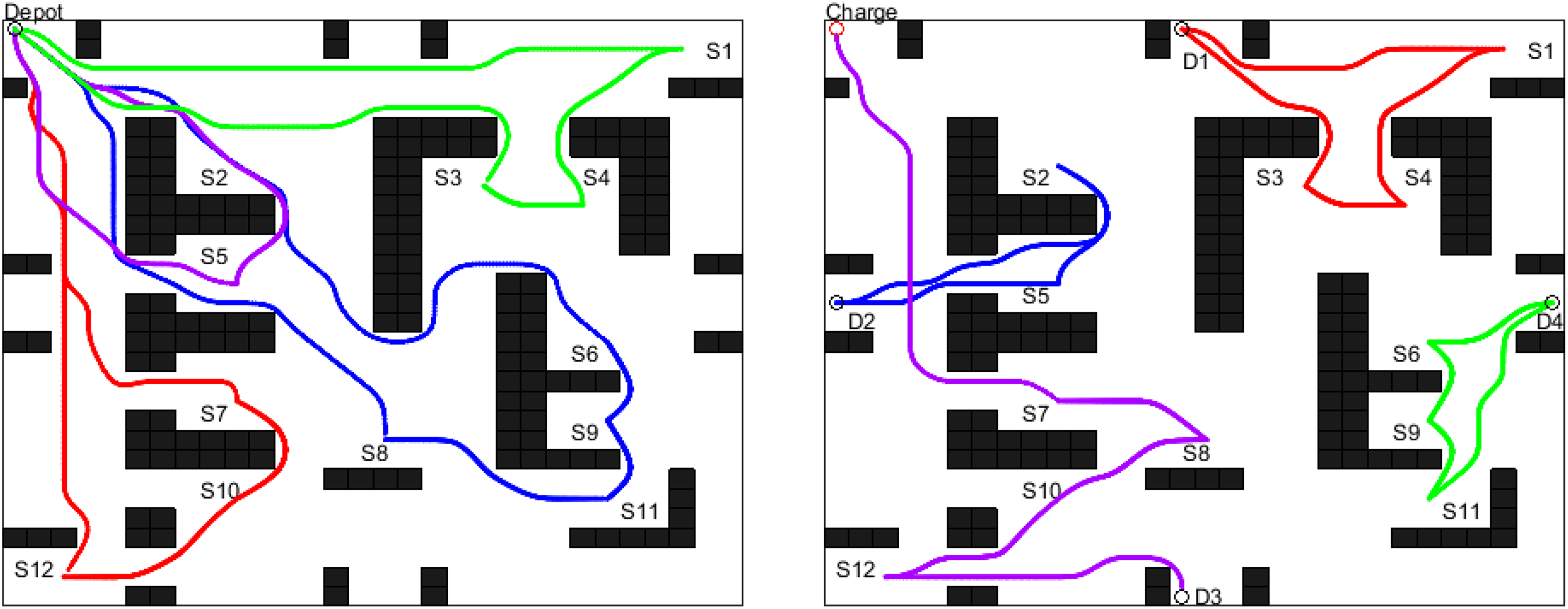
The actual path planning is performed by all AGV according to the scheduling results, which is shown in Figure 10. The comparison results of electricity consumption are recorded in Table 4.

Figure 10.

The actual routes of test 2.

Table 4.

Electricity consumption results of test 2.

AGV number	Single depot			Multi-depot
AGV number	Results without $ε_{2}$ (%)	Results with $ε_{2}$ (%)	Actual consumption (%)	Results without ${ε^{'}}_{2}$ (%)	Results with ${ε^{'}}_{2}$ (%)	Actual consumption (%)
1	10.46	13.91	12.09	3.78	4.69	4.01
2	9.11	12.12	13.32	5.83	7.23	7.83
3	5.53	7.36	9.14	9.15	11.35	11.96
4	14.72	19.58	18.40	5.18	6.42	6.82
Sum	39.82	52.97	52.95	23.94	29.69	30.62

AGV: automated guided vehicle.

In the case of the single depot, the actual total power consumption calculated by path planning is 52.95%. The result without $ε_{2}$ is 39.82%, which is 13.13% different from the actual one. Note that, the result with $ε_{2}$ is 52.97%, which is only 0.02% of the actual deviation. In the case of multiple depots, the actual total consumption is 30.62%. The total consumption is 23.94% without ${ε^{'}}_{2}$ , which is different from the actual consumption by 6.68%. And the result with ${ε^{'}}_{2}$ is 29.69%, which is only 0.93% different from the actual one.

Test 3: The last experiment with 12 stations is shown in map 3 of Figure 8. There are some discontinuous obstacles, which can provide passages for AGVs. Therefore, the map complexity coefficients of map 3 are $ε_{3} =1.29$ and ${ε^{'}}_{3} =1.22$ . The scheduling results as shown in Table 5. And the actual routes are shown in Figure 11. Table 6 shows the comparison results of electricity consumption.

Table 5.

The scheduling results of test 3.

AGV number	Solution routes of single depot	Solution routes of multi-depot
1	D→S12→S10→S7→D	D1→S3→S4→S1→D1
2	D→S8→S11→S9→S6→D	D2→S2→S5→D2
3	D→S2→S5→D	D3→S12→S10→S8→S7→C
4	D→S3→S4→S1→D	D4→S6→S9→S11→D4

AGV: automated guided vehicle.

Figure 11.

The actual routes of test 3.

Table 6.

Electricity consumption results of test 3.

AGV number	Single depot			Multi-depot
AGV number	Results without $ε_{3}$ (%)	Results with $ε_{3}$ (%)	Actual consumption (%)	Results without ${ε^{'}}_{3}$ (%)	Results with ${ε^{'}}_{3}$ (%)	Actual consumption (%)
1	10.83	13.97	14.05	6.00	7.32	7.67
2	12.97	16.73	16.60	4.83	5.89	6.19
3	5.98	7.71	7.00	10.00	12.20	11.43
4	10.66	13.75	14.16	4.44	5.42	5.26
Sum	40.44	52.16	51.81	25.27	30.83	30.55

AGV: automated guided vehicle.

In the case of the single depot of this test, the actual total electricity consumption is 51.81%. The result without $ε_{3}$ is 40.44%, but the result with $ε_{3}$ is 52.16%, which is 0.35% different from the actual one. For multi-depot, the result without ${ε^{'}}_{3}$ is 25.27%, and the results with ${ε^{'}}_{3}$ is 30.83%, which is very close to the actual consumption of 30.55%.

As one can see from the above examples, the developed scheduling method is quite reasonable and practicable for managing a fleet of AGVs. Note that, this method can accurately predict the power consumption of AGVs, and effectively allocate task or charging routes for AGVs.

Comparison with the algorithm

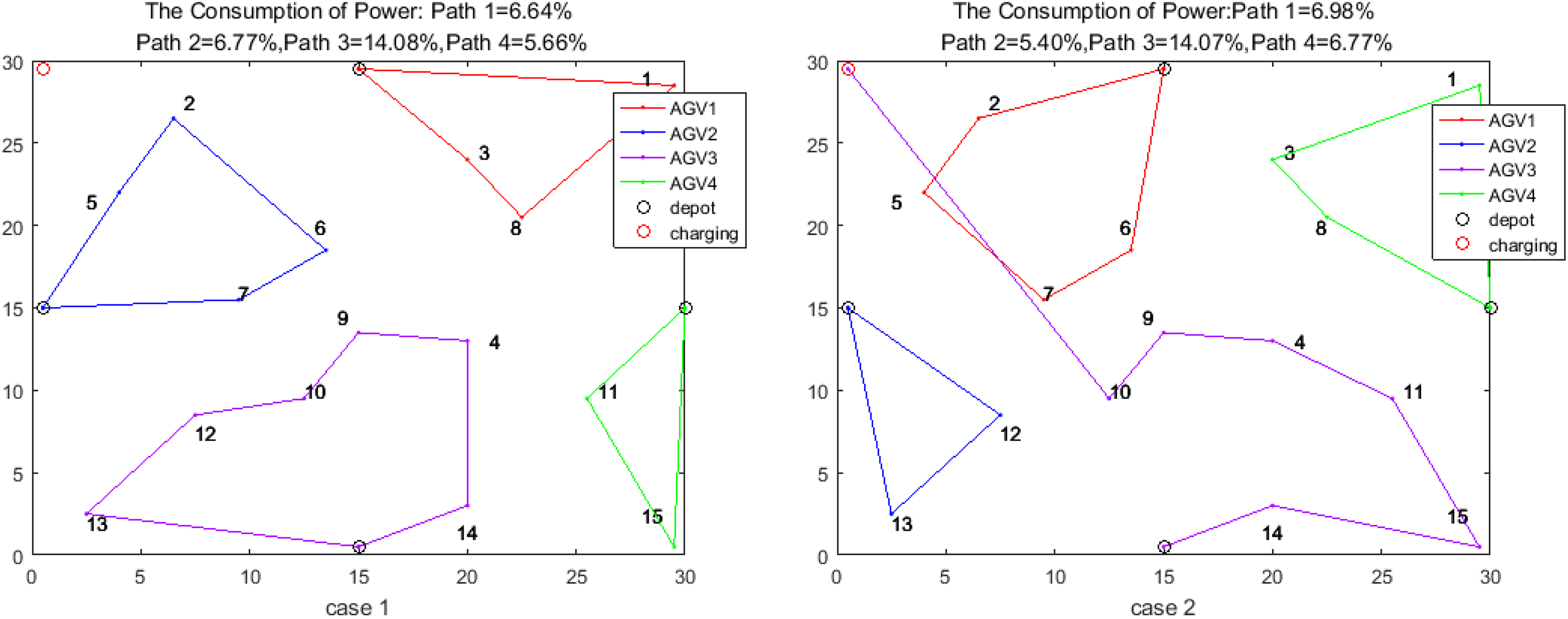
Furthermore, to reflect the importance of adding operation 1 and operation 2 in GA, this section compares the standard GA with the modified GAs that were illustrated in Figure 7. The GA control parameter settings are population size = 80 and the maximum number of generations = 500.

First, in the workshop environment with a single depot, arranging 5 AGVs to transport the materials, of which four AGVs have initial battery energy of 10% and another charge of 30%. The result of the standard GA is shown in case 1 of Figure 12, and the result of the GA with operation 1 is shown in case 2.

Figure 12.

The scheduling results of GA and GA with operation 1. GA: genetic algorithm.

As can be seen from Figure 12, the standard GA calculates that the power consumption of two routes has exceeded 10%, but there is only one AGV with more than 10% battery energy. The GA with operation 1 avoids such unreasonable results.

Next, in the workshop environment with multiple depots, arranging 4 AGVs with 20% battery charge to transport the materials. The value of the charge threshold of each AGV is set at 10%. The result of the standard GA is shown in case 1 of Figure 13, and the result of the GA with operation 2 is shown in case 2.

Figure 13.

The scheduling results of GA and GA with operation 2. GA: genetic algorithm.

As is shown in Figure 13, the GA with operation 2 can identify the AGV with lower power after the task is completed and assign it to the charging area.

Overall, the modifications of GA proposed in this article can obtain more reasonable scheduling results to ensure that the AGV have enough power to complete the task.

Conclusions

This article presented a new scheduling method for determining routes for multi-AGVs moving in 2-D workshop environments with a different number of depots. The scheduling model gives priority to the solutions with the minimum total power consumption of all AGVs and then selects the scheme that minimizes the makespan. To improve the multi-AGV scheduling method more practicable, a map complexity coefficient is derived according to the obstacles and depots’ number in the workshop. Then a modified GA is applied to the scheduling model to search for the reasonable routes. Experiments have shown good performance for this method. The method can make the scheduling results more practical without increasing the time complexity of the algorithm.

In the future, we plan to study extensions of the presented map complexity coefficient in a 3-D environment and consider the load capacity of AGV.

Footnotes

Declaration of conflicting interests

The author(s) declared no potential conflicts of interest with respect to the research, authorship, and/or publication of this article.

Funding

The author(s) disclosed receipt of the following financial support for the research, authorship, and/or publication of this article: This research is partly supported by the Common Key Technological Innovation Specialities of Key Industries of Chongqing Tongnan District Science and Technology Commission (Tk-2018-08), the National Natural Science Foundation of China (No. 51605064) and the Science and Technology Research Project of Chongqing Municipal Education Commission (No. KJ1600443).

ORCID iD

Fuli Wang

References

Yohanes

Khalfay

Nielsen

. Scheduling unmanned aerial vehicle and automated guided vehicle operations in an indoor manufacturing environment using differential evolution-fused particle swarm optimization. Int J Adv Robot Syst 2018; 15(1): 1–15.

Draganjac

Miklić

Kovačić

. Decentralized control of multi-AGV systems in autonomous warehousing applications. IEEE Trans Autom Sci Eng 2016; 13(4): 1433–1447.

Udhayakumar

Kumanan

. Task scheduling of AGV in FMS using non-traditional optimization techniques. Int J Simul Model 2010; 9(1): 28–39.

Anwar

Nagi

. Integrated scheduling of material handling and manufacturing activities for just-in-time production of complex assemblies. Int J Prod Res 1998; 36(3): 653–668.

Gnanavel Babu

Jerald

Noorul Haq

. Scheduling of machines and automated guided vehicles in FMS using differential evolution. Int J Prod Res 2010; 48(16): 4683–4699.

Pan

Zhang

. A case study of AGV scheduling for production material handling. Appl Mech Mater 2013; 414: 2351–2354.

Garey

Johnson

Sethi

. The complexity of flowshop and jobshop scheduling. Math Oper Res 1976; 1(2): 117–129.

Abdelmaguid

Nassef

Kamal

. A hybrid GA/heuristic approach to the simultaneous scheduling of machines and automated guided vehicles. Int J Prod Res 2004; 42(2): 267–281.

Murata

. Makespan minimization of machines and automated guided vehicles schedule using binary particle swarm optimization. Lec Note Eng Comput Sci 2010; 2182(1): 268–272.

10.

Rashmi

Bansal

. Task scheduling of automated guided vehicle in flexible manufacturing system using ant colony optimization. Int J Lat Tre Eng Tech 2014; 4(1): 177–181.

11.

Nishi

Maeno

. Petri net decomposition approach to optimization of route planning problems for AGV systems. IEEE Trans Autom Sci Eng 2010; 7(3): 523–537.

12.

Xidias

Zacharia

Nearchou

. Path planning and scheduling for a fleet of autonomous vehicles. Robotica 2016; 34(10): 2257–2273.

13.

Wang

Zhu

. Global path planning of wheeled robots using a multi-objective memetic algorithm. Integr Comput Aid Eng 2015; 22(4): 387–404.

14.

Vis

IFA

. Survey of research in the design and control of automated guided vehicle systems. Eur J Oper Res 2006; 170(3): 677–709.

15.

Xidias

Nearchouand

Aspragathos

. Vehicles scheduling in 2D shop floor environments. Indus Robot 2009; 36(2): 176–183.

16.

Xidias

Azariadis

. Mission design for a group of autonomous guided vehicles. Robot Auton Syst 2011; 59(1): 34–43.

17.

Azariadis

Aspragathos

. Obstacle representation by bump-surfaces for optimal motion planning. Robot Auton Syst 2005; 51(2–3): 129–150.

18.

Kawakami

Takata

. Battery life cycle management for automatic guided vehicle systems. In: Matsumoto

(eds) Design for Innovative Value Towards a Sustainable Society. Springer, 2012, pp. 403–408.

19.

Mousavi

Yap

Musa

. Multi-objective AGV scheduling in an FMS using a hybrid of genetic algorithm and particle swarm optimization. Plos One 2017; 12(3): e0169817.

20.

Čáp

Novák

Kleiner

. Prioritized planning algorithms for trajectory coordination of multiple mobile robots. IEEE Trans Autom Sci Eng 2015; 12(3): 835–849.

21.

Han

Wang

Liu

. Multi-AGV path planning with double-path constraints by using an improved genetic algorithm. Plos One 2017; 12(7): e0181747.

22.

Standley

. Finding optimal solutions to cooperative pathfinding problems. In: Proceeding of 24th AAAI Conference Artificial Intelligence (AAAI) (eds. Fox

Poole

), 2017, pp. 173–178.

23.

Wagner

Choset

. Subdimensional expansion for multirobot path planning. Artif Intell 2015; 219: 1–24.

24.

Erdmann

Lozano-Pèrez

. On multiple moving objects. Algorithmica 1987; 2: 1419–1424.

25.

Elfes

. Using occupancy grids for mobile robot perception and navigation. Computer 2002; 22(6): 45–67.

A novel scheduling method for automated guided vehicles in workshop environments

Abstract

Keywords

Introduction

Problem statement and mathematical formulation

Facility layout

Model derivation

The derivation of the map complexity coefficient

The modified genetic algorithm

Path planning

Experimental results and discussion

Analysis of proposed method validity

Comparison with the algorithm

Conclusions

Footnotes

Declaration of conflicting interests

Funding

ORCID iD

References