Sage Journals: Discover world-class research

Abstract

The performance of task-space tracking control of kinematically redundant robots regulating self-motion to ensure obstacle avoidance is studied and discussed. As the sub-task objective, the links of the kinematically redundant assistive robot should avoid any collisions with the patient that is being assisted. The shortcomings of the obstacle avoidance algorithms are discussed and a new obstacle avoidance algorithm is proposed. The performance of the proposed algorithm is validated with tests that were carried out using the virtual model of a seven degrees-of-freedom robot arm. The test results indicate that the developed controller for the robot manipulator is successful in both accomplishing the main-task and the sub-task objectives.

Keywords

Redundant Robot Manipulators Sub-task Control Self-motion Obstacle Avoidance Assistive Robots

1. Introduction

An exciting subset of service robotics research focuses on assistive robotics, resulting in several different robotic platforms being developed to assist disabled people [1]. The main aim of these systems is to provide support to a disabled person in his/her activities of daily living such as meal-serving and drink-serving, which are accomplished by using the semi-autonomous task execution principle (see Figure 1). It should be noted that a quadriplegic person is continuously inside the workspace of a robot arm during the application of this service robot.

Figure 1.

Overview of the FRIEND system [2]

Safety has been a significant concern during the development of service robots in each step of design iteratively to identify and assess the potential hazards. In addition, all aspects of the manipulator design, including the mechanics, electronics and software, should be considered [3]. Among these, in the complexity of a Human-Robot Interaction system (HRI), the physical viewpoint is mainly focused on the risks of collisions occurring between the robot arm and its user or, in this case, the patient. In such a scenario, the robot may cause serious harm or adverse effects to humans [3].

Since the most critical hazard can result from the collision of the robot arm with the user, the user area is usually separated from the robot workspace and, sometimes, it is monitored via two laser scanners, as it was done in the FRIEND system [1]. However, in the case of serving a meal to a quadriplegic person, the person is inside the workspace of the service robot, as shown in Figure 2. One possible approach is to reduce the power supply of the robot arm to provide safe operation near the user and minimize the transfer of energy/power to the user.

Figure 2.

Robot operation sequence for the “prepare and serve a meal” support scenario [2]

When there are obstacles, such as the human body within the workspace of a robot, another possible scenario is that the human body may collide with the links rather than the end-effector, since the desired end-effector pose trajectory is mostly chosen to avoid obstacles. In this case, obstacle avoidance algorithms are required to move the links away from the user while performing the main task. Since a kinematically redundant robot manipulator (or, in short, a redundant robot) has more DoF than required by its specified task [4], it can have an infinite number of possible configurations when tracking a given end-effector pose trajectory. According to the authors' best knowledge, Nakamura ‎[5] was the first researcher to name the motion of the links of a redundant robot that does not affect the end-effector motion as self-motion. This self-motion takes place in the null space of the redundant robot. In [30], an overview of the possible null space projections is provided. The null space projection used in this study is presented in Subsection 3.2. In addition to tracking a given end-effector pose trajectory, sub-tasks or secondary tasks can be accomplished by appropriately controlling the self-motion, which is usually called redundancy resolution. Generally, an objective function is defined to resolve the redundancy. The sub-tasks that have been widely investigated are obstacle avoidance ‎[6, 7], mechanical joint limit avoidance ‎[8] and the minimization of joint velocities or accelerations ‎[9].

Prior research addressed obstacle avoidance algorithm designs as a sub-task for redundant robots [10 –16] and a review of null-space. In these studies, the common approach was to first identify the closest points on the links of the redundant robot to the obstacles and then design a sub-task objective function to keep those points away from obstacles. In ‎[10] and ‎[11], one stationary obstacle was considered and the objective function to be maximized was chosen as the distance between the links of the redundant robot to avoid a collision. For the case of multiple obstacles, the objective function in ‎[10] and ‎[11] was modified in ‎[12] to be equal to the sum of the minimum distances to each obstacle. An alternative formulation in ‎[13] considered the square of the minimum distance as an objective function. Alternatively, ‎[14] preferred to utilize the reciprocal of the minimum distance as the objective function. Other studies, such as ‎[15], equipped a redundant robot with multiple proximity sensors to avoid collision with obstacles. However, as highlighted in ‎[16], utilizing the minimum distance in the objective function is problematic when there are multiple obstacles in the workspace of the robot.

A good review of existing methods for controlling redundant robots is given and the reviewed methods are examined in [29]. Since it was advised in [29] that, for redundant robots, task space control seems to be the most suitable control approach, in this study, a task-space controller derived from the work presented in [17] is used.

To address the lack of appropriate obstacle avoidance algorithms for redundant robots, this study aimed to formulate a novel obstacle avoidance sub-task objective function. Firstly, in Section 2, related works on obstacle avoidance are presented and the shortcomings of these are discussed. Before the description of the new method to provide a solution to these types of shortcomings, the kinematic and dynamic models of a redundant robot are given to form a base for the control design in Section 3. In Section 4, the feedback linearizing controller in ‎[17] is utilized to achieve the main control objective, which is tracking the desired end-effector pose trajectory. The controller includes an auxiliary term to fuse a sub-task controller for achieving a secondary objective, which, in this study, is obstacle avoidance. The general design of the objective function is also presented in Section 4. In Section 5, the new algorithm proposed in this study to compensate for the discussed shortcomings previous methods is described. Section 6 presents the results of the detailed numerical tests on the redundant robot used in the FRIEND system (LWA4-Arm by Schunk GmbH) to demonstrate the viability of the proposed obstacle avoidance algorithm. Depending on the given main task, this redundant robot may have several redundant (i.e., extra) DoF. Therefore, it has more flexibility in terms of possible configurations than a planar scenario. In the first set of numerical tests, two obstacles are used to evaluate the difference of the new algorithm with the existing algorithm. Later, numerical tests for a single obstacle are presented to evaluate the performance of the new algorithm and the parameters that affect this performance. This paper is finally concluded with discussions on the test results.

2. Related Work on Obstacle Avoidance Sub-task Formulation

The purpose of the obstacle avoidance sub-task formulation is to select an objective function that keeps the closest points of the links to the obstacles away from the selected obstacles. Among the various studies carried out on this topic, the most common methodology for avoiding obstacles is to optimize an objective function using the self-motion of the redundant robot while completing the main-task.

Generally, an objective function is chosen in relation to the minimum distance between the links of the redundant robot and the obstacles. The simplest objective function is obtained by setting $f (q) = d$ which is to be maximized ‎[10, 11]. Considering multiple obstacles in the workspace of a redundant robot, the objective function $f (q)$ can be modified as a sum of the minimum distances, as shown below ‎[12]

f (q) = \sum_{i = 1}^{n_{o}} \sum_{j = 1}^{n} d_{i j} (q)

(1)

where $d_{i j}$ is the minimum distance between i^th link and j^th obstacle, and n and n_o are the total number of links and obstacles, respectively. In another formulation by ‎[13], the square of the minimum distance is used as an objective function. One alternative approach is to use the reciprocal of the minimum distance, as in ‎[14].

For all of the mentioned objective functions, as discussed in ‎[16], there are several shortcomings of using the minimum distance, especially when there is more than one obstacle. In Figure 3.a, points P₁, P₂ and P₃ represent the point obstacles that lie on the same line perpendicular to the link. The minimum distances from P₁, P₂ and P₃ to the link are calculated as d₁, d₂ and d₃, respectively. For a finitely small amount of counter-clockwise rotation δq₁ for the joint variable, q₁, δd₁, δd₂ and δd₃ can be written as

Figure 3.

Point type of obstacles near the link: (a) P1, P2 and P3 lie on the same line; (b) P1 and P2 lie on the same line; (c) P1 is closer than P2 to the centre of rotation [16]

\frac{δ d_{1}}{δ q_{1}} = \frac{δ d_{2}}{δ q_{1}} = - \frac{δ d_{3}}{δ q_{1}} = O C .

(2)

In view of (2), it is clear that, for a small amount of joint motion, all of the obstacles occurring along the same line perpendicular to the i^th link have the same norm of distance gradient with respect to q_i regardless of the distance between the link and the obstacle (which is equal to the projection of the obstacles to the link or in this case, $O C$ ). Therefore, when considering the multiple obstacles P₁ and P₂ - as illustrated in Figure 3.b - the minimum distance based objective functions cannot provide a decision for obstacle avoidance priority, simply because both gradients are of the same norm and opposite direction. Therefore, the decision to rotate clockwise or counter-clockwise for the next motion can be made in either direction. In this case, obstacle P₁ becomes more critical for a possible collision with this algorithm.

In the configuration presented in Figure 3.c, P₁ is closer to the link and its probability of collision with the link is higher. However, the objective function in (1) will drive the first link in the counter-clockwise direction, which results in an increase in d₂ since the gradient of d₂ is greater than that of d₁. This problem gets even worse when the objective function is chosen as the square of the minimum distances since its gradient is now weighted by each distance. As such, obstacle P₂ has the dominant gradient (d₂∇d₂) over P₁ (d₁∇d₁). Even if the objective function is selected as the reciprocal of the distances, there will be problems. Consider the case where d₁ and d₂ are the same for the configuration in Figure 3.c, ( $d_{2} / d_{2}^{2}$ ) gradient is higher than ( $d_{1} / d_{1}^{2}$ ) gradient and will result in a motion towards the P₁ obstacle. This can cause critical situations when these two obstacles are very close to the link and a small joint motion would result in a collision with one of them.

3. Model of the Redundant Robot

In this section, the kinematic and dynamic models of the redundant robot, along with the model properties, are given. In this work, an n -DoF robot with the dimension of its workspace being m is considered with $n > m$ , thus resulting in a redundant robot application.

3.1. Kinematics model

The end-effector position $p (q) \in ℜ^{l}$ and orientation $ϕ (q) \in ℜ^{(m - l)}$ in the task (operational) space are the components of the task space pose, denoted by $x (t) \in ℜ^{m}$ . This is obtained as a function of joint position vector as

x = k (q) = [\begin{matrix} p (q) \\ ϕ (q) \end{matrix}]

(3)

where $k (q) \in ℜ^{m}$ denotes the forward kinematics and $q (t) \in ℜ^{n}$ denotes the joint position vector. The forward kinematics in velocity level is obtained by differentiating the forward kinematics in (3) as

\overset{\cdot}{x} = J (q) \overset{\cdot}{q}

(4)

where $J (q) = \partial k (q) / \partial q \in ℜ^{m \times n}$ is the Jacobian of the redundant robot, $\overset{\cdot}{q} (t) \in ℜ^{n}$ denotes the joint velocity vector, while $\overset{\cdot}{x} (t) \in ℜ^{m}$ is the end-effector velocity vector. It is highlighted that, since $n > m$ , the Jacobian matrix J is not square. Thus, its inverse does not exist. Differentiating the velocity kinematics in (4) yields

\overset{\cdot\cdot}{x} = \overset{\cdot}{J} (q) \overset{\cdot}{q} + J (q) \overset{\cdot\cdot}{q}

(5)

where $\overset{\cdot\cdot}{q} (t) \in ℜ^{n}$ denotes the joint acceleration vector and $\overset{\cdot\cdot}{x} (t) \in ℜ^{m}$ is the end-effector acceleration vector. From (4) and (5), the inverse relations on velocity and acceleration levels can be obtained as

\overset{\cdot}{q} = J^{+} \overset{\cdot}{x} + {\overset{\cdot}{θ}}_{N}

(6)

\overset{\cdot\cdot}{q} = J^{+} (\overset{\cdot\cdot}{x} - \overset{\cdot}{J} \overset{\cdot}{q}) + {\overset{\cdot\cdot}{θ}}_{N}

(7)

where ${\overset{\cdot}{θ}}_{N} (t) \in ℜ^{n}$ and ${\overset{\cdot\cdot}{θ}}_{N} (t) \in ℜ^{n}$ are projections of joint velocity and acceleration vectors onto the null space of the Jacobian. The pseudo-inverse denoted by $J^{+} \in ℜ^{n \times m}$ is defined as in ‎[18, 19] by

J^{+} = J^{T} {(J J^{T})}^{- 1}

(8)

when J has full rank (i.e., the manipulator is not in a singular configuration). Notice that $J^{+}$ satisfies $J J^{+} = I_{m}$ where I_m is an m × m identity matrix. Other matrix relations that are satisfied by pseudo-inverse and its null space projection are given in Appendix A.

3.2. Dynamic model

The dynamic model for an n-link, all revolute-joint robot manipulator has the following form ‎[20]

M (q) \overset{\cdot\cdot}{q} + C (q, \overset{\cdot}{q}) + G (q) + F (\overset{\cdot}{q}) + ξ_{d} = τ

(9)

where $M (q) \in ℜ^{n \times n}$ represents the generalized inertia matrix, $C (q, \overset{\cdot}{q}) \in ℜ^{n}$ represents the torques due to centripetal-Coriolis effects vector, $G (q) \in ℜ^{n}$ is the gravitational effects on the joints vector, $F (\overset{\cdot}{q}) \in ℜ^{n}$ represents the frictional effects vector, $ξ_{d} (t) \in ℜ^{n}$ is a vector containing bounded, unknown and additive disturbance effects, and $τ (t) \in ℜ^{n}$ is the joint torque input vector. It is noted that the inertia matrix is positive definite and its inverse exists for all $q (t)$ ‎[21].

4. Control Objective

The tracking objective is to design the torque input vector $τ (t)$ so that the end-effector of the redundant robot tracks the desired end-effector pose as closely as possible. In addition, the control input should be designed to include the necessary components to execute sub-tasks defined by an optimization measure to make use of the extra DoF of the redundant robot. From now on, the task space tracking will be referred to as the main-task objective and the optimization measure for self-motion as the sub-task objective. In one of the previous studies by Shen et al. [28], obstacle avoidance is applied in numerical simulations on a seven DoF robot manipulator. However, the control is accomplished in the kinematic level, unlike the control presented in this paper.

4.1. Main-task control objective

Since the main aim of this study is to design an obstacle avoidance sub-task and better present the performance of the proposed sub-task function, accurate knowledge of the kinematic and dynamic models are assumed, along with the availability of full-state feedback (i.e., joint position vector and joint velocity vector are available).

To quantify the task space tracking objective, tracking error, denoted by $e (t) \in ℜ^{m}$ , is defined as

e = x_{d} - x

(10)

where $x_{d} (t) \in ℜ^{m}$ is the desired position defined in task space and $x (t) \in ℜ^{m}$ is the sensory feedback of the joint position. The control input torque $τ (t)$ is formulated as ‎[17]¹

τ (t) = M_{c} {J^{+} ({\overset{\cdot\cdot}{x}}_{d} + K_{v} \overset{\cdot}{e} + K_{p} e - \overset{\cdot}{J} \overset{\cdot}{q}) + {\overset{\cdot\cdot}{θ}}_{N}} + N_{c}

(11)

where K_v and K_p are constant, positive definite, diagonal gain matrices, $M_{c} (q)$ is the calculated generalized inertia matrix, $N_{c} (q, \overset{\cdot}{q})$ is the calculated nonlinear terms that appear in the dynamics equation of the robot (i.e., $C (q, \overset{\cdot}{q}), G (q), F (\overset{\cdot}{q}), ξ_{d}$ ), and ${\overset{\cdot\cdot}{θ}}_{N}$ , introduced in (7), is a joint acceleration vector projected onto the null space of J, which is yet to be designed, If the manipulator does not go through a singularity, then the control law in (11) guarantees that the tracking error converges exponentially to the origin. While a similar proof of convergence for the tracking error can be found in ‎[17], it is demonstrated in Appendix B for the sake of completeness.

4.2. Sub-task control objective

Consider a vector function $g (q, t) \in ℜ^{n}$ that may be a function of time and/or joint positions. The sub-task control objective is to make the null space projection of the joint velocity vector ${\overset{\cdot}{θ}}_{N}$ to track the projection of g onto the null space of J. Since $(I - J^{+} J)$ projects vectors onto the null space of J, the above objective can be quantified as a null space velocity tracking error, denoted by ${\overset{\cdot}{e}}_{N} (t) \in ℜ^{n}$ , as

{\overset{\cdot}{e}}_{N} = (I - J^{+} J) g - {\overset{\cdot}{θ}}_{N} .

(12)

The auxiliary control term ${\overset{\cdot\cdot}{θ}}_{N}$ that is utilized to integrate the sub-task objective into the control input torque is designed as ‎[17]

{\overset{\cdot\cdot}{θ}}_{N} = (I - J^{+} J) \overset{\cdot}{g} - (J^{+} \overset{\cdot}{J} J^{+} + {\overset{\cdot}{J}}^{+}) J g + K_{N} {\overset{\cdot}{e}}_{N}

(13)

where K_N is a constant, positive definite and diagonal gain matrix. Taking the time derivative of the null space velocity tracking error in (12) results in

{\overset{\cdot\cdot}{e}}_{N} = (I - J^{+} J) \overset{\cdot}{g} - ({\overset{\cdot}{J}}^{+} J + J^{+} \overset{\cdot}{J}) g - {\overset{\cdot\cdot}{θ}}_{N}

(14)

and then substituting the auxiliary controller in (13) yields in

{\overset{\cdot\cdot}{e}}_{N} = - J^{+} \overset{\cdot}{J} g + J^{+} \overset{\cdot}{J} J^{+} J g - K_{N} {\overset{\cdot}{e}}_{N} .

(15)

In view of the closed-loop null space velocity tracking error in (15), the auxiliary controller in (13) ensures that the joint velocities in the null space converge to $(I - J^{+} J) g$ , provided that the vector function g and its time derivative are designed to be bounded (the proof is provided in Appendix C).

4.3. Sub-task objective function

The projection of the vector function g onto the null space of J can be considered as the desired null space joint velocities, which will be designed to accomplish a given sub-task. To control the self-motion of the redundant robot, the vector function g is designed as

g = k \nabla f

(16)

where $\nabla f (q)$ is the gradient of the objective function $f (q)$ , and k is a scalar gain.

In the next sections, related work on an obstacle avoidance sub-task and the new formulation for an obstacle avoidance sub-task are described in detail.

5. New Algorithm for Obstacle Avoidance

The objective of this sub-task is to keep the closest point on the links away from the selected obstacles. The first step involves the calculation of distance and its unit vector direction by finding the location of the point X_Cij (called the critical point c) on each link i =1,2,‥, n that is nearest to the obstacles (the obstacle number is given by j=1,2,…, $n_{o}$ ). This can be done by a set of geometric calculation procedures ‎[22] and this algorithm can be executed for each link and each obstacle.

Since exact trajectory tracking for the critical point with respect to obstacles is not in question, a simple obstacle avoidance scheme can be achieved by means of the Jacobian matrix transpose method ‎[23, 24];

{\overset{\cdot}{q}}_{c} = \sum_{i = 1}^{k} \sum_{j = 1}^{n} J_{c i}^{T} (q) v_{c i j}

(17)

where $v_{c i j}$ is the obstacle escape velocity. The escape velocity can be set by the user to regulate the self-motion speed. In the next section, tests are conducted to observe the effect of selecting different escape velocities. Once the obstacle escape velocity, $v_{c i j}$ is determined, it can be transformed to the joint space by (17). This vector will be used as the gradient of the objective function ( $g = {\overset{\cdot}{q}}_{c}$ ) to avoid obstacles. This way of formulation resolves the problems faced with the previous obstacle avoidance algorithms, since the gradient of the objective function is not used but g is calculated directly without using (16).

In this method, the escape velocity $v_{c i j}$ can be defined as a function of the minimum distance $d_{i j}$ along the direction away from the critical point X_Cij

v_{c i j} = v_{m} exp (- d_{i j}) u_{i j} .

(18)

In (18), v_m is the maximum escape velocity scalar and $u_{i j}$ is the unit vector from the critical point X_Cij on the i^th link to the j^th obstacle. The selection of v_m and the exponential relation between the escape velocity and the minimum distance affects the performance of the self-motion for obstacle avoidance. As a result of utilizing the exponential function, when $d_{i j}$ is sufficiently large, no collision danger exists and this results in $v_{c i j}$ being smaller. On the contrary, when $d_{i j}$ is getting small (closer to zero), then additional safety action needs to be taken while holding $v_{c i j}$ with its maximum norm value ( $v_{c i j} = v_{m}$ ) and thus, the sub-task objective is reached. Among previously developed algorithms, the most convenient obstacle avoidance algorithm, which is devised by taking the reciprocal of the distances, results in limitless null space velocity demands if no precaution is taken. However, the speed of the change in escape velocity is exponential and the selected exponential function never goes over the selected v_m value. This is essential to limiting the motor torque demands during operation.

When the proposed formulation is analysed for a spatial robotic arm, it can be shown that it has two drawbacks:

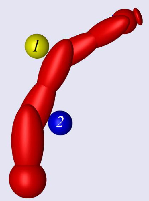
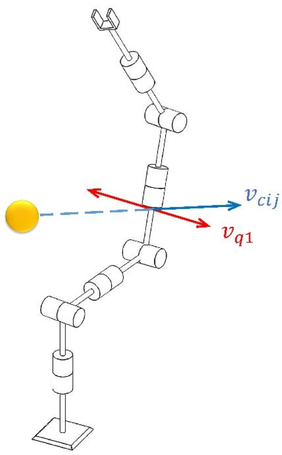
The first drawback happens when the obstacle and robot arm are situated in such a position that the escape velocity vector $v_{c i j}$ is perpendicular to the instantaneous velocity vector generated for the i^th link for any joint motion. An example of such a case is given in Figure 4 for the motion of the fourth link with respect to the first joint's motion.

Figure 4.

Sketch of the robot arm when the escape velocity of a link is perpendicular to the instantaneous motion of the same link with respect to a joint motion

In the case defined in Figure 4, the calculated velocity of the first joint in the null space to move the fourth link away from the obstacle will be zero. As a result, there will be no sensation in that joint to that obstacle. This critical scenario will continue unless the end-effector trajectory in the main task goes through a motion that changes this perpendicular angle of the velocity vectors. The possible collision scenario for this specific case is simulated in Figure 5 as a sequence of motion captures. In Figure 5, the robot link's visual representation is shown with red ellipsoids. The obstacle is the yellow circle. The blue arrow shows the direction of the task space motion of the end-effector. It can be observed that the collision happens at the 12^th second.

Figure 5.

Sequence of motion captures for the special case scenario

The second drawback is valid for all of the mentioned obstacle avoidance techniques. It is when the minimum distance between the obstacle and the link intersects with the imaginary extension of that link at the critical point X_Cij, as shown in Figure 6. In this case, the related link will still be moved to avoid the obstacle, despite the fact that it is not likely to collide with the j^th obstacle.

Figure 6.

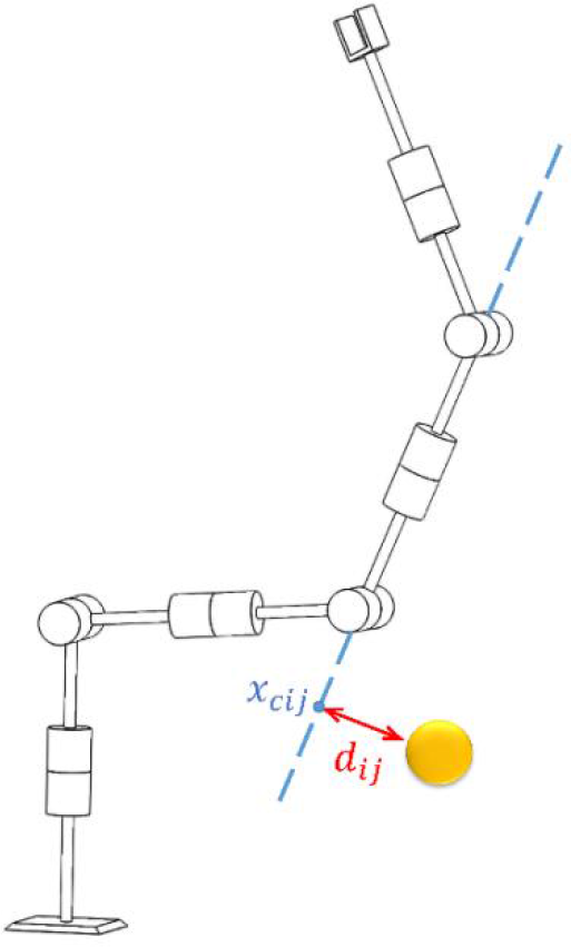
Sketch of the robot arm when the distance of a link from the obstacle is calculated with respect to the extension of a link

6. Simulation Results

To illustrate the performance of the proposed obstacle avoidance sub-task objective function for the self-motion control of redundant robots, a set of detailed numerical test results are presented. In these tests, the virtual model of 7 DoF LWA4-Arm manufactured by Schunk GmbH is used. For simulation purposes, the dynamic and kinematics models of the 7 DoF LWA4-Arm are obtained by using the method described in ‎[25] in two stages. First, the robot arm is modelled by SolidWorks software with respect to the CAD data provided in ‎[26], as shown in Figure 7. Then, the CAD model is exported in 3D XML format to MATLAB Simulink by using the plug-in, SimMechanics Link. As a result of the transfer of the model from CAD environment to SimMechanics, the model could be used for numerical tests to evaluate the performance of the proposed obstacle avoidance algorithm.

Figure 7.

The CAD Model of 7-DoF LWA4-Arm

The second stage includes the modelling of the control system and development of the necessary kinematics and dynamic equations of the robot by using MATLAB Simulink blocks that are based on the kinematics of the robot defined in Table 1. The visualization tools of SimMechanics are also used to display and animate 3D robot geometries, before and during simulation.

Table 1.

Denavit-Hartenberg parameters of LWA4-Arm

i	θ_i	d_i(m)	#x03B1;_i(rad)
1	θ₁ (q₁)	0.3	π/2
2	θ₂(q₂)	0	− π/2
3	θ₃(q₃)	0.328	π/2
4	θ₄(q₄)	0	− π/2
5	θ₅(q₅)	0.317248	π/2
6	θ₆(q₆)	0	− π/2
7	θ₇(q₇)	0	0

The numerical tests were conducted with MATLAB Simulink with a fixed-step sample time of 0.1 kHz. The manipulator is considered to be initially at rest at the joint positions q= [0 −25 0 −35 0 −10 0]^T in degrees.

In the first set of simulation tests, the new algorithm presented in this paper is evaluated against a previously developed algorithm. With the next set of simulation tests, the new algorithm performance and the parameters that affect this performance are evaluated.

6.1. Test results to compare the previous algorithms and the new algorithm

This set of tests is conducted to compare the new algorithm performance with the previously presented methods. As a representative of the previously developed methods, the objective function is selected as the reciprocal of the minimum distance between obstacles and the nearest point on the link. In this case, $(d_{2} / d_{2}^{2}) + (d_{1} / d_{1}^{2})$ is selected as the gradient.

In order to compare the new algorithm with the older ones, two obstacles are located within the workspace of the robot arm at ob₁ = [0.04 0 0.65]^T and ob₂ = [0.14 0 0.32]^T, as shown in Figure 8.

Figure 8.

Two obstacles placed inside the robot's workspace

The main task of the selected manipulator is to hold its tip point position at a constant location. In this case, the robotic arm will only perform a motion in its null space. A constraint is formulated so that the manipulator moves as if it is a planar 3-DoF arm in the plane presented in Figure 8. In order to simulate planar arm motion, joints one, three, five and seven are fixed and only joints two, four and six are controlled for the task. The distance of link two with respect to the obstacles is initially kept as do₁ and do₂ at 71.66 and 78.43 mm, respectively.

The next figures reveal the difference between the two methods. In Figure 9, the sub-task controller with the proposed obstacle avoidance sub-task formulation in (17) and (18) are used. It can be observed that the distances between obstacle one and link two (do₁) and the distance between obstacle two and link two (do₂) are balanced in the time at relevantly similar distances.

Figure 9.

Distance of link two to obstacle one and two by using the new algorithm

When the reciprocal of the minimum distances algorithm is used, the test concludes with link two moving much closer to obstacle two, as depicted in Figure 10. This is because the distance rate of do₁ was initially larger than that of do₂, similar to the case described in Figure 3.c.

Figure 10.

Distance of link two to obstacle one and two by using the reciprocal of distances method

6.2. Performance evaluation tests of the new algorithm

A common benchmark test for all simulations is designed and Figure 11 shows the desired task-space trajectories for this test. The trajectory is selected to track the positions only in the Cartesian space without constraining the orientation of the end-effector.

Figure 11.

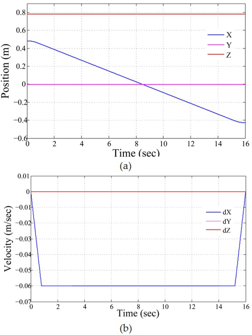
Desired task-space trajectories: (a) desired position trajectory, (b) desired velocity

For this scenario, the manipulator had four extra DoF than the required DoF to perform the main objective. This gave the robot manipulator increased flexibility when carrying out the task used to execute obstacle avoidance as a sub-task.

In the controller presented in (11), the nonlinear terms, which include centripetal and Coriolis $C (q, \overset{\cdot}{q})$ , frictional $F (\overset{\cdot}{q})$ and disturbance ξ_d terms, are neglected for simplicity reasons and only gravitational effects are used to compensate the nonlinear effects (i.e., gravity compensation). We would like to note that this simplification was considered because the robot moves in slow motion, which induces a modelling error that must be compensated by the controller.

The control gain matrices, K_v, K_p and K_N are tuned iteratively and set to have values of 200, 200 and 170 for each element on the diagonal respectively in order to obtain acceptable end-effector tracking performance for the given task. The sub-task objective function parameter v_m was chosen as 20 when the obstacle was located at $X_{O} = {[0 - 0.06 0.6]}^{T}$ .

Figure 12 shows the end-effector tracking errors during simulation, which are the main task errors. From this result, it can be observed that the end-effector position tracking error remained within a small bound of less than 0.2 mm after four seconds. This indicates that the main-task objective is successfully achieved. The larger error at about one second is due to a sudden configuration change, which is discussed later in this paper.

Figure 12.

Main-task error calculated with respect to the measured end-effector trajectory

The joint velocities for numerical simulation are given in Figure 13. The joint velocities, except the ones during the time interval between zero and two seconds, are observed to be larger than if the sub-task was chosen as the minimization of the joint velocities. When the manipulator is away from the obstacles, the escape velocity is minimized but it does not go to zero. Thus, the joint velocities may receive higher magnitudes in achieving this sub-task.

Figure 13.

Joint velocities measured during the simulation

The importance and the effect of assigning sub-task objective can be observed from the measured joint velocities in Figure 13. After the first second, a sudden change of configuration can be observed. This sudden configuration change results in higher velocity demands at the joint level. Since the designed controller does not account for the velocity-related nonlinear effects, such as Coriolis and centripetal effects, the faster motion demand results in larger main-task trajectory tracking errors. This can be observed at the same time intervals in Figure 12. The sudden configuration change is illustrated in Figure 14 with screenshots taken during the simulation. It is observed from the screenshots that the sudden configuration change initiated at second 1 and terminated at second 1.8. The blue line in the screenshots indicates the direction of end-effector position trajectory, which is the main task of the manipulator. It is important to observe the total motion from the top view in Figure 14.b to see that the obstacle is not penetrated but the manipulator moves around the obstacle.

Figure 14.

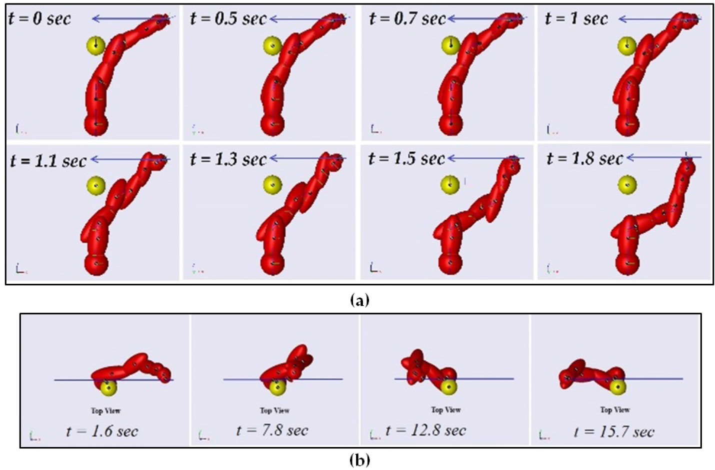
Sequence of motion captures: (a) Sudden configuration change of the manipulator, (b) Total task from top view

Figure 15 is presented to indicate the performance of the controller for sub-task execution. The sub-task error given in Figure 15 is the norm for ${\overset{\cdot}{e}}_{N}$ and it is practically regulated and stays bounded, which indicates that the sub-task objective is achieved. Configuration changes can also be clearly observed in Figure 15, since the errors rise at the first second.

Figure 15.

Norm of null space velocity tracking error

In the previous figures, the simulation results are presented for a selected escape velocity of 20 m/s. In order to investigate the effect of the escape velocity selection, a number of simulation tests are carried out. The escape velocity is varied from 0.1 to 20 m/s. The results for the obstacle avoidance performance can be investigated for all of the links. However, only the second link's behaviour is provided in this paper due to page limitations. In Figure 16, the vertical axis is the distance of the second link to the obstacle. It can be observed that at about the first second, for the escape velocities that are lower than 5 m/s, the second link almost collides with the obstacle. In fact, when the escape velocity is 0.1 m/s, the second link collides with the obstacle. However, since there is no collision model in the simulation when the collision happens, the second link moves through the obstacle.

Figure 16.

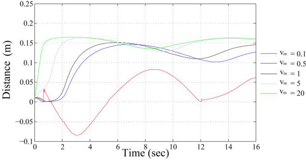
Distance between the second link and the obstacle during the same task for different escape velocity values

While the escape velocity is varied in the previous case, the main task speed is selected to be the same for all cases. In the next simulation tests, the aim is to investigate the effect of the main task speed on a selected escape velocity. The escape velocity is selected to be 5 m/s for this investigation since 5 m/s is the critical escape velocity to move the second link away from the obstacle for the specific example. The maximum task speeds in the trapezoidal velocity trajectory presented in Figure 11.b are selected as 0.06, 0.24 and 0.48 m/s. The results for these main task speeds are presented in Figure 17. In order to have a fair judgment between the performances with different main task speeds, the horizontal axis of the plot is selected to be the measured end-effector position. The motion initiates at about 0.49 m for all of the cases and the end-effector moves in the (–) x-axis. It is observed from Figure 17 that, as the main task speed is increased, the distance between the second link and the obstacle becomes smaller. Therefore, increasing the main task speed for the same escape velocity increases the chance of a collision with the obstacle.

Figure 17.

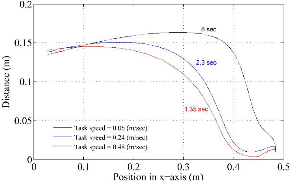
Distance between the second link and the obstacle for different task velocities when escape velocity is selected as 5 m/s

7. Discussions and Conclusions

In this paper, a new obstacle avoidance objective function is designed that utilizes the self-motion of a redundant robot to avoid contact with obstacles within its workspace. The main motivation of designing a new obstacle avoidance objective function for redundant robots is the shortcomings of the objective functions that are currently available in literature. Specifically, in previous literature, the common method is to introduce an objective function that is formed by the minimum distance between the links of the redundant robot and the obstacles. However, when the minimum distance based objective functions are utilized for multiple obstacles, as demonstrated in Section 4, the above-presented algorithms may fail to provide the priority of which obstacle will be avoided first. Subsequently, while trying to avoid the obstacle that is located further away, a collision of the robot with the obstacle that is closer to the base may be unavoidable. This is an important problem for service robots, where the obstacle to avoid is usually the operator/user.

In the new algorithm that is proposed in this work, in a novel departure from the existing research, an exponential function of the distance between the obstacles and the links was utilized. Numerical tests were performed by using the virtual model of a 7 DoF LWA4-Arm to validate the proposed obstacle avoidance objective function. In the first numerical tests, the new algorithm was tested against an existing algorithm in which the reciprocal of the distances method is used. The new algorithm provided better results in terms of keeping link two in similar distances away from both obstacles. In the next set of numerical tests, the main-task was achieved, where the end-effector tracking error remained within the magnitude of 1 mm, while the links of the redundant robot successfully avoided the obstacle.

Another issue addressed in this work is the selection of the escape velocity in the developed obstacle avoidance algorithm. A number of simulation tests were carried out to investigate the effects of selecting a different escape velocity while the main task speed is constant and selecting different main task speeds while the escape velocity is constant. The results indicated that lower escape velocities might result in the collision of the links with the obstacles. However, the suitable magnitude of the escape velocity to successfully avoid obstacles is also related with the main task execution speed. Therefore, it can be concluded that the escape velocity should be selected with respect to the task execution speed and it can be adjusted during online trajectory planning scenarios.

We would like to note that the main motivation of this study was the design of a novel obstacle avoidance objective function. In lieu of the main motivation, the exact model knowledge was considered to be available, along with full-state feedback, and the feedback linearizing controller in ‎[17] was utilized. In this manner, we demonstrated the performance of the proposed obstacle avoidance objective function. However, when there are structured/parametric uncertainties in the dynamics, the previous work of the third author ‎[8], which is the least-squares based adaptive version of ‎[17], can also be utilized. Another previous work of the third author, in ‎[27], a gradient-based Lyapunov-type version of the controller in ‎[17] could have also been utilized. Finally, if there are unstructured uncertainties in the dynamics, then the robust controller in ‎[15] can be utilized.

Footnotes

8. Acknowledgements

This work is supported in part by The Scientific and Technological Research Council of Turkey via (grant number 113E147).

1

A slight modification of the feedback linearization controller in ‎[17] is utilized to achieve task-space tracking. The main reason for the preference of the controller in () is to better demonstrate the performance of the novel sub-task obstacle avoidance objective function.

Appendix A

The pseudo-inverse also satisfies the following

(19)

J J^{+} J = J

(20)

J^{+} J J^{+} = J^{+}

(21)

{(J^{+} J)}^{T} = J^{+} J

(22)

{(J J^{+})}^{T} = J J^{+}

while the projection matrix onto the null space of the Jacobian satisfies

(23)

{(I - J^{+} J)}^{T} = (I - J^{+} J)

(24)

(I - J^{+} J) (I - J^{+} J) = (I - J^{+} J)

(25)

(I - J^{+} J) J^{+} = 0.

Appendix B

The closed-loop error system is given by

(26)

M \overset{\cdot\cdot}{q} + N = M_{c} {J^{+} ({\overset{\cdot\cdot}{x}}_{d} + K_{v} \overset{\cdot}{e} + K_{p} e - \overset{\cdot}{J} \overset{\cdot}{q}) + {\overset{\cdot\cdot}{θ}}_{N}} + N_{c} .

By assuming that we can calculate the generalized inertia matrix and nonlinear terms in the dynamic equation with some precision ( $M_{c} ≅ M$ and $N_{c} ≅ N$ ), the above expression can be simplified to

(27)

\overset{\cdot\cdot}{q} = J^{+} ({\overset{\cdot\cdot}{x}}_{d} + K_{v} \overset{\cdot}{e} + K_{p} e - \overset{\cdot}{J} \overset{\cdot}{q}) + {\overset{\cdot\cdot}{θ}}_{N}

where the positive definiteness of the inertia matrix was also utilized ‎[21]. Equating (27) and (7) results in the following closed-loop error system

(28)

\overset{\cdot\cdot}{e} + K_{v} \overset{\cdot}{e} + K_{p} e = 0

where $J J^{+} = I$ was utilized. The proper choice of diagonal elements of K_v and K_p with $s^{2} + K_{v} s + K_{p}$ being a Hurwitz polynomial in Laplace variable s in (28) implies that the task space tracking error e goes to zero exponentially.

Appendix C

It is first noted that, ${\overset{\cdot\cdot}{θ}}_{N}$ in (13) belongs to the null space of J since $J {\overset{\cdot\cdot}{θ}}_{N} = 0$ after utilizing

(29)

J (I - J^{+} J) = 0

(30)

J (J^{+} \overset{\cdot}{J} J^{+} + {\overset{\cdot}{J}}^{+}) = \frac{d}{d t} (J J^{+}) = \frac{d}{d t} (I) = 0

(31)

J K_{N} {\overset{\cdot}{e}}_{N} = 0.

Define a non-negative scalar Lyapunov function, denoted by $V_{N} ({\overset{\cdot}{e}}_{N})$ , as the half of the norm square of the null space velocity tracking error as

(32)

V_{N} = \frac{1}{2} {\overset{\cdot}{e}}_{N}^{T} {\overset{\cdot}{e}}_{N} .

The time derivative of the Lyapunov function in (32) is equal to

(33)

{\overset{\cdot}{V}}_{N} = {\overset{\cdot}{e}}_{N}^{T} {\overset{\cdot\cdot}{e}}_{N}

and after substituting (15) into the above expression and after straightforward mathematical manipulations, it can easily be obtained that

(34)

{\overset{\cdot}{V}}_{N} = - {\overset{\cdot}{e}}_{N}^{T} K_{N} {\overset{\cdot}{e}}_{N} .

In view of $V_{N} ({\overset{\cdot}{e}}_{N})$ in (32) and ${\overset{\cdot}{V}}_{N} ({\overset{\cdot}{e}}_{N})$ in (34), it is easy to see that ${\overset{\cdot}{e}}_{N}$ is asymptotically driven to the origin.

The null space velocity tracking error in (12) can alternatively be rewritten as

(35)

{\overset{\cdot}{e}}_{N} = (I - J^{+} J) (g - \overset{\cdot}{q})

from which it is easy to see that the joint velocities in the null space of J track the projection of g onto the null space of J.

References

Graser

Heyer

Fotoohi

Tange

Kampe

Enjarini

Heyer

Fragkopoulos

Ristic-Durrant

: A Supportive FRIEND at Work: Robotic Workplace Assistance for the Disabled. Robotics and Automation Magazine IEEE. 2013;20.4: 148–159. DOI: 10.1109/MRA.2013.2275695.

Grigorescu

Lüth

Fragkopoulos

Cyriacks

Gräser

: A BCI-controlled Robotic Assistant for Quadriplegic People in Domestic and Professional Life. Robotica. 2012; 30.03: 419–431. DOI: 10.1017/S0263574711000737.

Alami

Albu-Schaeffer

Bicchi

. Safe and Dependable Physical Human-robot Interaction in Anthropic Domains: State of the Art and Challenges. In: International Conference on Intelligent Robots and Systems; 9–15 October 2006; Beijing China. 2006. p. 1–16.

Conkur

Buckingham

: Clarifying the Definition of Redundancy As Used in Robotics. Robotica. 1997; 15: 583–586.

Nakamura

. Advanced Robotics: Redundancy and Optimization. 1st ed. Boston: Addison-Wesley Longman Pub. Co. Inc.; 1991. 337 p.

Baillieul

. Avoiding Obstacles and Resolving Kinematic Redundancy. In: IEEE 1986 International Conference on Robotics and Automation; 7–10 April 1986; San Francisco, CA, USA: IEEE; 1986. p. 1698–1704.

Colbaugh

Seraji

Glass

: Obstacle Avoidance for Redundant Robots Using Configuration Control. International Journal of Robotic Systems. 1989; 6: 721–744. DOI: 10.1002/rob.4620060605.

Tatlicioglu

Braganza

Burg

Dawson

: Adaptive Control of Redundant Robot Manipulators with Sub-task Objectives. Robotica. 2009; 27: 873–881. DOI: 10.1017/S0263574708005274.

Seraji

. Task Options for Redundancy Resolution Using Configuration Control. In: 30th IEEE Conference on Decision and Control; 11–13 December 1991; Brighton, England: IEEE. p. 2793–2798.

10.

Guo

Hsia

. Joint Trajectory Generation for Redundant Robots in an Environment with Obstacles. In: IEEE 1990 International Conference on Robotics and Automation; 13–18 May 1990; Cincinnati, OH, USA: IEEE. p. 157–162.

11.

Wang

Hamam

: Optimal Trajectory Planning of Manipulators with Collision Detection and Avoidance. International Journal of Robotics Research. 1992; 11: 460–468. DOI: 10.1177/027836499201100503.

12.

Kemeny

: Design and Evaluation Environment for Collision-free Motion Planning of Cooperating Redundant Robots. Periodica Polytechnica Ser El. Eng. 1999; 43:189–198.

13.

Chen

Liu

Lee

Liang

: On-line Multi-criteria Based Collision-free Posture Generation of Redundant Manipulator in Constrained Workspace. Robotica. 2002; 20: 625–636. DOI: 10.1017/S0263574702004204.

14.

Chung

Lee

. Obstacle Avoidance for Kinematically Redundant Robots Using Distance Algorithm. In: IROS'97 the 1997 IEEE/RSJ International Conference on Intelligent Robots and Systems; 7–11 Sep 1997; Grenoble, France: IEEE. p. 1787–1793.

15.

Kapadia

Tatlicioglu

Dawson

D. M.

. Set-point Navigation of a Redundant Robot in Uncertain Environments Using Finite Range Sensors. In: Proceedings of IEEE International Conference on Decision and Control; 9–11 December 2008; Cancun, Mexico: IEEE. p. 4596–4601.

16.

Lee

Buss

. Obstacle Avoidance for Redundant Robots Using Jacobian Transpose Method. In: IROS 2007 IEEE/RSJ International Conference on Intelligent Robots and Systems; 29 Oct – 2 Nov 2007; San Diego, CA, USA: IEEE. p. 3509–3514.

17.

Hsu

Mauser

Sastry

: Dynamic Control of Redundant Manipulators. Journal of Robotic Systems. 1989; 6: 133–148. DOI: 10.1002/rob.4620060203.

18.

Golub

Van Loan

: Matrix Computations. 1st ed. Baltimore: The John's Hopkins University Press; 1983.

19.

Yoshikawa

. Analysis and Control of Robot Manipulators with Redundancy. In: Robotics Research: The First International Symposium; 1984; Cambridge, MA, USA: MIT Press. p. 735–747.

20.

Spong

Vidyasagar

: Robot Dynamics and Control. 1st ed. New York: John Wiley & Sons; 1989. 336 p.

21.

Tewis

Dawson

Abdallah

: Robot Manipulator Control: Theory and Practice. 2nd ed. New York: Marcel Dekker; 2004. 638 p.

22.

Maaroof

OWN

. Self-motion Control of Kinematically Redundant Robot Manipulators [Thesis]. Izmir, Turkey: Izmir Institute of Technology; 2012.

23.

Sciavicco

Siciliano

: Solution Algorithm to the Inverse Kinematic Problem for Redundant Manipulators. IEEE Journal of Robotics and Automation. 1988; 4: 403–410. DOI: 10.1109/56.804.

24.

Das

Slotine

Sheridan

. Inverse Kinematic Algorithms for Redundant Systems. In: IEEE 1988 International Conference on Robotics and Automation; 24–29 April 1988; Philadelphia, PA, USA:IEEE. p. 43–48.

25.

Dede MIC: Virtual Prototyping of Robot Controllers. International Journal of Design Engineering. 2010; 3: 276–288. DOI: 10.1504/IJDE.2010.039761.

26.

Schunk GmbH. LWA4-Arm CAD Drawings [Internet]. 2015. Available from: http://www.schunk-modular-robotics.com/left-navigation/service-robotics/service-download/simulationcad/cad-data.html. Accessed on 21 Sep 2015.

27.

Tatlicioglu

Mcmtyre

Dawson

Walker

: Adaptive Nonlinear Tracking Control of Kinematically Redundant Robot Manipulators. International Journal of Robotics and Automation. 2008; 23: 98–105. DOI: 10.2316/Journal.206.2008.2.206-3081.

28.

Shen

Chen

Jiang

Yan

: Obstacle Avoidance Algorithm for 7-DOF Redundant Anthropomorphic Arm. Journal of Control Science and Engineering. 2015; 2015, 1–9. DOI: 10.1155/2015/540259

29.

Nakanishi

Cory

Mistry

Peters

Schaal

: Operational Space Control: A Theoretical and Empirical Comparison. The International Journal of Robotics Research. 2008; 27(6): 737–757. DOI: 10.1177/0278364908091463.

30.

Dietrich

Ott

Albu-Schäffer

: An Overview of Null Space Projections for Redundant, Torque-Controlled Robots. The International Journal of Robotics Research. 2015; 34(11): 1385–1400. DOI: 10.1177/0278364914566516.

A New Objective Function for Obstacle Avoidance by Redundant Service Robot Arms

Abstract

Keywords

1. Introduction

2. Related Work on Obstacle Avoidance Sub-task Formulation

3. Model of the Redundant Robot

3.1. Kinematics model

3.2. Dynamic model

4. Control Objective

4.1. Main-task control objective

4.2. Sub-task control objective

4.3. Sub-task objective function

5. New Algorithm for Obstacle Avoidance

6. Simulation Results

6.1. Test results to compare the previous algorithms and the new algorithm

6.2. Performance evaluation tests of the new algorithm

7. Discussions and Conclusions

Footnotes

8. Acknowledgements

1

Appendix A

Appendix B

Appendix C

References