Sage Journals: Discover world-class research

Abstract

In recent years, several important advances have been made in the fields of both biologically inspired sensorial processing and locomotion systems, such as Address Event Representation-based cameras (or Dynamic Vision Sensors) and in human-like robot locomotion, e.g., the walking of a biped robot. However, making these fields merge properly is not an easy task. In this regard, Neuromorphic Engineering is a fast-growing research field, the main goal of which is the biologically inspired design of hybrid hardware systems in order to mimic neural architectures and to process information in the manner of the brain. However, few robotic applications exist to illustrate them. The main goal of this work is to demonstrate, by creating a closed-loop system using only bio-inspired techniques, how such applications can work properly. We present an algorithm using Spiking Neural Networks (SNN) for a biped robot equipped with a Dynamic Vision Sensor, which is designed to follow a line drawn on the floor. This is a commonly used method for demonstrating control techniques. Most of them are fairly simple to implement without very sophisticated components; however, it can still serve as a good test in more elaborate circumstances. In addition, the locomotion system proposed is able to coordinately control the six DOFs of a biped robot in switching between basic forms of movement. The latter has been implemented as a FPGA-based neuromorphic system. Numerical tests and hardware validation are presented.

Keywords

Address Event Representation Neuromorphic Systems Dynamic Vision Sensors Biped Robot Locomotion Spiking Neurons

1. Introduction

Spiking Neural Networks (SNN) comprise an information-processing paradigm inspired by the ways in which biological nervous systems, such as the brain, process information [1]. In this regard, electronic and computer engineers contribute to our understanding of the brain's computation as follows [2]:

Developing sensors, data-processing algorithms and simulation platforms used by computational neuroscientists.

Undertaking research that links empirical neuroscience evidence with hypotheses about how neurobiological systems manipulate information.

Imitating biological-computation mechanisms in specific applications, e.g., robotic systems.

The algorithm proposed in this work is inspired by the idea that biological cortical structures are composed of a small number of processing layers, and that neurons of the visual cortex are selectively sensitive to the orientation of the lines and edges in the visual field.

Interpreting visual stimuli in human or animals might appear to be an effortless process, but this is because its complexity is far from being fully understood. However, huge efforts and advances have been made for this cause in the last few decades. Between 1950 and 1960, Hubel and Wiesel's study of cats found that neurons of the visual cortex are selectively sensitive to the orientation of lines and edges in the visual field [3, 4].

Later, inspired by the works of Hubel and Wiesel, the concept of cognition was introduced by Fukushima in [5] and improved in [6]. It consists of a multilayered structure that is self-organized by “learning without a teacher”, and acquires an ability to recognize stimulus patterns based on the geometrical similarity (Gestalt) of their shapes without being affected by their positions. The principles of such papers have served as inspiration for the techniques used in Address Event Representation (AER) cameras. We also note that a cell has synapses that are afferent only from a group of cells situated in a particular area predetermined for each cell. This area is named the connectable area of the cell, which is determined by the spread of the dendrites and of the axon terminals of each cell.

Besides these features, biological cortical structures are composed of a small number of processing layers, no more than 10, where a wavefront of spikes crosses from the sensing layer to the resulting layer while different operations are performed, as explained by [7]. For different applications, each layer has a specific goal. For example, for characters' detection, the kernel of a layer might be focused on deleting background noise and, in some other applications, on detecting clusters of data, straightness or curved lines, etc. Such techniques are favourable in the sense that tolerating a small positional error at a given time at each stage, rather than all in one step, plays an important role in endowing the network with the ability to recognize even distorted patterns [8].

Conventional image-processing techniques are based on the principle that a video recorder registers a given number of images per second, which, when played in sequence, make up a video. These images are usually called frames and their rates can vary depending on the application: between 30 and 60 frames/second are used in most of the conventional applications. Various important techniques have been successfully developed for pattern recognition, e.g., examining colour or texture in images. Using frames implies that the sensor must register a whole image each time, line by line, which can prove to be a restriction on the speed of the processing.

In recent years, a different approach to the problem has begun to grow in popularity. It uses Dynamic Vision Sensors (DVS) that do not depend on frames, but rather on registering changes of lighting in specific sections of the area being sensed, and on using the coordinates of such an area, or pixel, to perform the processing. Under this logic, assuming that the background is fixed to some extent, events will only be registered when a movement is detected. This technology is commonly known as Address Event Representation (AER); it uses mixed analogue and digital principles and exploits pulse-density modulation for coding information, as explained in [9]. A difficulty of pattern recognition techniques lies in separating the important data from the noise and background. This is bypassed to some extent in AER sensors, where only the areas in which light changes are detected, registered and transmitted.

Current DVSs work within a range of resolution around 128×128 pixels, usually giving as the output the address of the pixels that were activated – a sign indicating whether it was a positive or negative change in the lighting – and giving a time stamp of the event [7, 10, 11]. These events are registered into a buffer, which waits until it is full and then proceeds to be transmitted to a CPU for processing. Some examples of applications tested by Address Event Representation techniques are: the tracking of vehicles on a highway, presented in [12]; a robot arm that acts as a football goalkeeper by blocking incoming balls in [13]; a robot that uses AER auditory sensory input to feedback its central pattern generator [14] and a pencil balancer [15]. This last example requires a very fast response, providing a good demonstration of the fast-response capabilities of AER; usually, position encoders are used to make this kind of control.

Once the events are registered, diverse processing methods can be applied to extract the useful information. For example, clusters of events are formed around an object of interest, such as a ball or a car in the road. A moving edge will tend to produce events that are correlated closer in time with nearby events from the same edge; as opposed to noise, that tends to be more erratic and not easily correlated with neighbours or with past events for the same pixel [16].

2. Materials

Most robots that are designed for the purpose of line following are wheeled, which in itself simplifies a lot of the stability and the dynamics of the movements. Basic vision sensors are normally used, generally only in order to detect drastic changes in the lighting and give an on/off output per sensor. Considering such circumstances, it was decided to follow this principle and to implement a feedback system for line following for a biped robot. In broad terms, the tasks required were:

Understanding and reading properly the events coming from the AER sensor for processing.

Events-based processing using a spiking neural network for the approximation and tracking of the line's position.

Giving the appropriate orders to the biped robot in order for it to remain in the line's path.

2.1. The Biped Robot

A considerable variety of biped robots with different configurations and that are mainly driven by servomotors are available, making their control very practical and straightforward. For this work, we used the Biped BRAT robot shown in Figure 1, manufactured by the company Lynxmotion. It has a configuration of six motors, three in each leg, meant to represent the ankle, knee and hip joints. A servomotor controller, provided by the same manufacturer, is also used; the SSC-32, with 32 channels and a resolution of 1 mS, acts as an intermediate step in the communication between the designed system and the servomotors. Because of this, the developed system needs only to provide as an output a serial command coded in ASCII to the SSC-32 Controller, which then transforms it into a Pulse-Width Modulation (PWM) signal for each servomotor.

Figure 1.

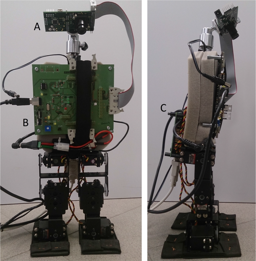
Biped robot with AER sensor and USBAERmini2 board

The Biped BRAT is assembled in such a way that a PWM pulse of 1.5 mS in each of its servomotors corresponds to the Home Position, with the biped standing up. When using the SSC-32 Controller for a given servomotor, one unit change in the position value corresponds to a 1 mS change in the PWM pulse. An example of a command that sends the robot to its Home Position is #0P1500 #1P1500 #2P1500 #16P1500 #17P1500 #18P1500 T1000. This is read by the SSC-32 Controller as the order in which to set the motors connected to the ports numbered 0, 1, 2, 16, 17 and 18, to a pulse width of 1.5 mS.

2.2. The USBAERmini2 Communication Board

The USBAERmini2 is a low-cost, high-speed USB2.0 AER interface implemented in [17]. This interface allows real-time capturing of AER communication, as well as AER event sequencing with event rates of up to four mega-events per second. It also introduces the capability to capture events synchronously from several devices. It features three parallel AER ports: one for sequencing, one for monitoring and one for passing through the monitored events. In [18], the author describes the USBAERmini2 as a bridge between a USB port and AER buses. It is able to monitor AER traffic trough the USB port, and also to sequence AER information.

2.3. The jAER Software

jAER is a Java software project that allows soft real-time, event-driven processing AER systems on PCs. It is centred around an application named jAERViewer, that allows the user to plug in an AER device with a USB interface, view the events coming from the device, log them to disk, play them back and process them, as explained in [16]. In the website [19], an open-source repository of Java and Matlab functions can be found, along with some sample data files containing recordings of AER sensors – for example, the recording of the movement of a hand or an outdoors environment. Some of the provided Matlab functions were used in the development of this work.

3. Methodology

As mentioned previously, the general goal of this project is to gain an understanding and to apply some of the concepts of Neuromorphic Engineering, such as how Spiking Neural Networks behave and the use of Dynamic Vision Sensors. This task could also be solved by purely geometrical or mathematical methods, but it is proposed as a demonstration of the capabilities and flexibility of this research area, in an attempt to apply it to a structure similar to one that can be found in nature, such as legged locomotion.

3.1. Biped Robot Walking

By observing the movement of different robot models and by testing a sequence of commands, we have enabled the robot to make basic movements: taking a step forwards or backwards, or making a left or right turn. In broad terms, the idea behind the movements is rather symmetrical. When it is desired to take a step either forwards or backwards, the robot needs to place its center of mass in only one of the legs, allowing the second one to move freely; this takes a couple of commands. The robot is then free to make the second leg move forwards and to switch the center of mass to the other leg; this is mostly done by movements in the ankle joints. When this step is completed, the robot can then continue with a second step, turning in a circle or returning to the home position. Preserving the symmetry of the movements is very convenient.

In Figure 2, a diagram with all the possible combinations of positions that can take place is presented; each one of the movements (forwards, backwards, turn left and right) takes a total of nine commands in different combinations. The one labelled “Home” is the start and end of each step taken. Positions “Balance1” and “Balance2” normally occur in sequence and they are designed to place the robot's center of mass on the right leg, leaving the left leg off the ground and free to move forwards or backwards. Positions “Balance3” and “Balance4” are equivalent, but invert the function of each leg. Positions “Walk1” to “Walk4” are mainly focused on putting one leg forwards, then switching the center of mass to said leg, followed by making the second leg catch up with the previous one. The two remaining positions have a function similar to the one previously described, with the difference that they are made while both legs are supporting the weight of the robot. The friction with the ground while the movement takes place enables the robot to switch its facing direction towards one of the sides. These position areas are called in different sequences, depending on the desired movement of the robot.

Figure 2.

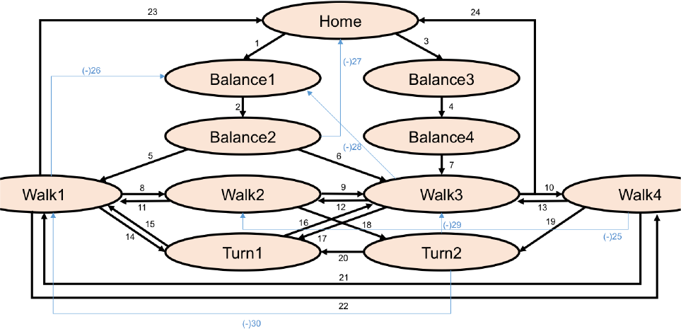
Diagram of all the possible sequences of positions required for the movements

3.2. Processing AER Data by Layers

During the walking of the robot, even waking in a straight line, its movements change the vision range of the sensor drastically. In Figure 3, we show a series of screenshots recorded by the AER sensor mounted on the robot when approaching a curve to the left while following a straight line and when approaching a curve to the right, respectively. Since some of the movements are made more quickly than others, sometimes the line is very easy to identify. On some occasions, however, the line is almost completely faded, so the processing has to be broad enough to compensate for it.

Figure 3.

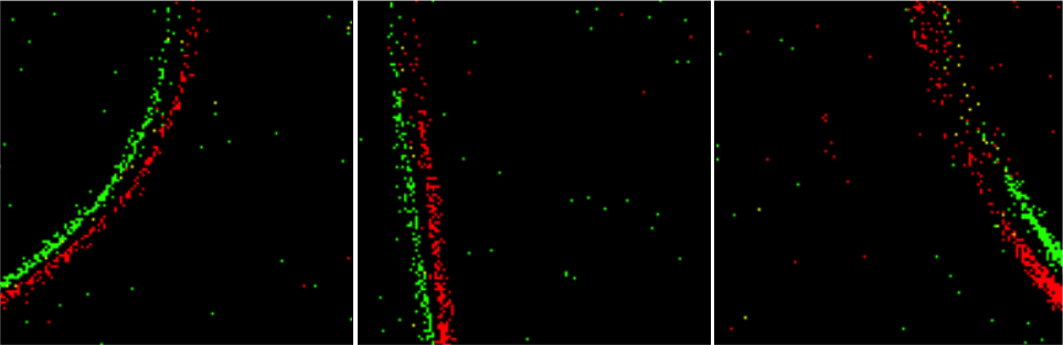
Three sample screenshots from an AER sensor mounted on the biped

This work was developed mostly under Matlab, since a lot of the tools that this platform required for the control of the Dynamic Vision Sensor were available in open-source forms. Nevertheless, it was also considered to be an interesting goal in order to understand how a simple Spiking Neural model could be implemented in VHDL and to understand its implications. This was tested using pre-recorded data from the vision sensor and processed under simulation. The information obtained can then be programmed into a FPGA in order to command a sequence of movements to the robot and enable it to move without an attached computer. The AER camera used has a resolution of 128×128 pixels; each time an event occurs, it is registered in 8 bytes, i.e., an int32 address word and an int32 time stamp.

A couple of pictures of the complete biped robot and the sensor configuration are presented in Figure 1. The main electronic components are:

A: 128×128 AER retina sensor.

B: USBAERmini2 board.

C: SSC-32 Controller servomotor.

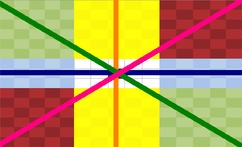
With the goal of following the principles of biomorphic robotics – trying to emulate the mechanics, sensor systems and computing methodologies found in biological organisms – our approach consists of a series of layers, shown in Figures 4 and 5. The AER retina sensor itself is represented as the first layer, with a resolution of 128×128 pixels. The second one is a 16×16 layer of neurons, using a simple Integrate-and-Fire model. Each one of the 256 neurons receives as an input the accumulated number of events detected in the corresponding 8×8 region of the sensor data. This fulfils the function of downsizing the input data, as well as eliminating a lot of the noise generated by events that are not highly correlated to others in their proximities.

Figure 4.

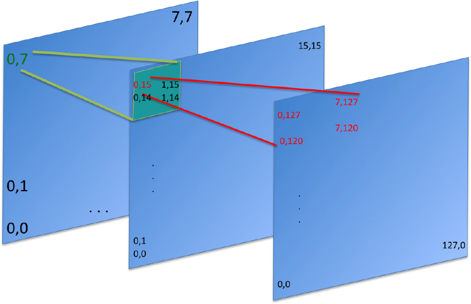
First three processing layers of the AER events for line detection

Figure 5.

Transition between the third and fourth layers of processing

In addition, the third layer consists of downsizing, in this case to an 8×8 matrix, where each element simply adds the activations detected in the neurons of the second layer, in a region of 2×2 neurons. Once the 8×8 layer is processed, the next step is to detect which one of the 64 possible segments received the most activations, under the assumption that it represents part of the tracked line. Following these steps, by this point we would know the coordinates of a point that is part of the line with a resolution of 8×8. Therefore, in order to obtain a complete approximation of the line, according to its equation, we only need to know a second point or its slope (m).

The fourth layer has the goal of detecting the most probable slope that corresponds to the line. It consists of a set of neurons, each one representing a specific slope, where the one that gives the most activations is considered to be the winner and, for our purposes, completing the determination of the line's position. Given that the biped robot can only make a series of basic movements (making a step forwards or backwards, and turning to each side), it was decided to use four possible slopes, thus using only four neurons: one for a horizontal line ( $m = 0$ ), one for a vertical line (slope undefined due to its division by zero), and a couple of neurons for slopes $m = 1$ and $m = - 1$ . This means that we have a total of 64 possible points that are part of the line, and four possible slopes for each of them – meaning 256 results, bearing in mind that a lot of these results correspond to the same line and were simply detected as starting from a different point. This resolution could be modified for a better approximation of the line's position, following the same principle.

The distribution of how the 8×8 layer data is transmitted to the fourth layer is in a function in which the point that detected most activations in the previous layer is found. A point of the line detected in a corner of the layer cannot provide the same distribution of input to the next layer as a point that is found in the opposite corner. For this reason, a larger 15×15 layer is used; if the center of the said layer is matched with the most active point in the 8×8 layer, then all possible distributions are covered. Figure 6 gives a representation of the 15×15 layer, where each colour represents one of the four neurons. Figure 7 gives three examples of how the output of the 8×8 layer can be placed as an input in the subsequent one, according to the most active point, represented in this case by the black square. It is easy to make the deduction that the slope corresponding to the neuron that receives more inputs and ends up winning is also a function of the said position.

Figure 6.

Fourth layer: slope approximation

Figure 7.

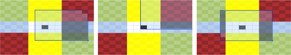
Examples of fitting in the last layer

3.3. The Neuron Model

The Leaky Integrate-and-Fire (LIF) neuron is probably the best-known example of a formal spiking neuron model, [20]. For this work, a simplified version is implemented, as described in Equations 1 to 3.

V_{m} (t) = V_{m} (t - 1) + \frac{V - V_{m} (t - 1)}{τ_{m}}

(1)

V_{o} = (\begin{matrix} V_{m} (t) + V_{s p i k e} & if V_{m} (t) \geq V_{t h} \\ 0 & if V_{m} (t) < V_{t h} \end{matrix}

(2)

t_{r e s} = {\begin{matrix} τ_{r} & if V_{m} (t) \geq V_{t h} \\ 0 & if V_{m} (t) < V_{t h} \end{matrix}

(3)

In Table 1, a summary of the representation and initial values of the variables can be consulted.

Table 1.

Parameters of the LIF neuron model

Variable	Description	Initial value (and units)
τ _m	=R_mC_m*; time constant	8 (msec)
τ _r	Refractory period	4 (msec)
V _th	Spike threshold	1 (volts)
V _spike	Voltage spike	0.5 (volts)
V_m(t)	Membrane voltage	(volts)
V_m(t−1)	Previous membrane voltage	(volts)
V_o	Output voltage	(volts)
t _res	Resting time	(msec)
V	Input voltage	(volts)

3.4. Switching between Recording, Processing and Decision Taking

Since the recording of data events is done using jAER, and the data processing is done using Matlab, autonomous communication between them is required. jAER is configured by default to be able to receive instructions using the User Datagram Protocol (UDP), under which one computer application can send messages to another. With a few lines of code, Matlab can instruct jAER to start recording a file of the events and then instruct the file to be closed. This has the inconvenience that the processing is not done in real time; a file that is recording events needs to be closed in order to start reading them from the beginning. However, for this specific application, this methodology can still be used. Since it takes the robot a few seconds to complete the sequence of commands corresponding to a step or a turn, it only needs to make a decision at the end of said movement. The main idea of the implementation is that events are recorded during the first half of each steep, a file containing them is saved and, during the second half, the events are read from the file and processed. At the end, the best approximation of the line is chosen, the decision is taken and the loop is then ready to start the process again for the next step. This also has the advantage that the events can be posteriorly consulted and reproduced, even when the camera and the USBAERmini2 board are not attached to the robot. Since each step is saved as a separate file, the sequence of events that led up to a decision being made by the robot is also clear. The robot can then re-enact a trajectory, and posterior experimentation with it is possible.

For the first step, the robot needs to be taken out of its motionless position so that events can be detected by the sensor. For this reason, an extra sequence of movements was added: that of balancing the robot in its place. This is specified as the starting sequence, and the first step is only made after enough events have been registered by the algorithm to make an estimation of the line. This sequence is also entered in the case when the line is not inside the vision field of the sensor. In summary, at the end of each step, the robot can decide between five sequences of movements: taking a step forwards, turning left or right, taking a step backwards or balancing in its place. Not all the movements take the same time to complete, and not all of them are equally likely to happen, since the weights for the neurons that choose to take a turn are set to be bigger. The step backwards is very unlikely to happen, as it has far fewer events that are set as inputs and their weights are smaller, but in certain cases, it does help the robot to get return to the path after getting lost. Finally, the balancing sequence is entered by default when no neurons of the last layer are activated.

4. Results

A few links to sample videos of the robot's behaviour are included in section 6 of this document. The question of how to choose a fair quantitative analysis of the robot's decision-making process is not trivial; a lot of factors need to be taken into account. For instance, a proper adjustment of the robot needs to be made before its operation; since only a low-cost tripod was used to mount the AER sensor onto the robot, it was easy to accidentally derange its orientation. It was found that when the camera faced the floor too directly, sometimes the proper decisions were not taken in time. When a curve was detected, the robot would take a step too late, and by the time that the movement was completed, the line might already be outside of the vision field of the robot. In addition, the feet of the robot would sometimes get into the said vision field, and the events generated would interfere with the line estimation. Conversely, if the sensor's orientation is too upright, segments of the line path that are not being tracked currently get in the way; this is caused because the curvature of the path causes parts of the line to be close to each other.

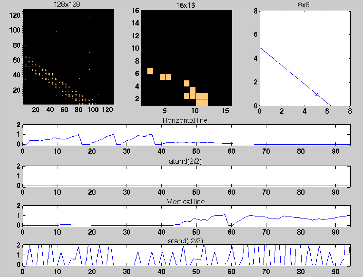
Another aspect that needs to be taken into account is the complexity of the said path. In this case, it was already available and had been used previously in other applications. It consists of a continuous line with a few intersections and turns to both sides, see Figure 8. For the nature of the implementation, we believe that interruptions or dotted parts of the line would not only not prejudice but also help in line detection, since more events would be generated by the sensor, caused by lighting changes. Figures 9 and 10 show two illustrations of how the position of the line is detected in Matlab: the first one when it is a straight line, and the second one when a turn to the left is required. In each of these two figures, the top three panels display the activated neurons for the layers of 128×128, 16×16 and 8×8 neurons, respectively. The lower four panels show the activations for the horizontal lane: the one curved to the right, the vertical line (meaning a forwards path) and the line curved to the right, respectively.

Figure 8.

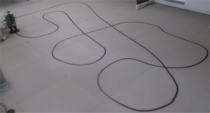
Line path used to test the biped robot

Figure 9.

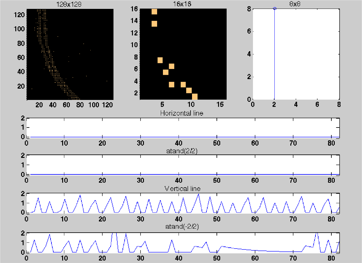
Matlab program detecting a straight line

Figure 10.

Matlab program detecting a line curved to the left

It is not possible to completely predict what line the robot will follow in the case of intersections. In most cases, however, it is not the one in front but one of the turns, since a new line entering the vision field will always cause new events other than the one that was already being followed. Due to the dynamics of the robot, a single wrong decision would cause the line to be outside of the sensor's vision field, and, in consequence, preventing it from being able to take any more decisions. For this reason, in a lot of the tests, the robot ends up losing track of the line after about three to five minutes. Counter-intuitively, more difficulties were faced in the parts of the path with a long straight line, since the system detects that a step forwards is required but, not being an ideal system, with the centre of mass not completely centred and not entirely symmetrical, the robot's direction deviates a little with each step while detecting the line as straight. Eventually, after a long sequence of only forwards steps, around seven to 10, the line ends up being outside of the vision field. From a total of 30 trials recorded for analysis, the robot takes an average of 20.6 decisions before taking a wrong turn that prevents it from keeping track of the line. This takes an average of 3:41 minutes, regardless of the starting point. Figure 11 shows the number of decisions before making a wrong turn for a sample of 30 tests, as well as the time required for some of them.

Figure 11.

Table showing the number of decisions before making a wrong turn for a sample of 30 tests, as well as the time required for some of them

5. Discussion

This work consisted in the synergy of several techniques and technologies, whose implications need to be taken into account. Some of these features contrasted very highly with each other. Probably the main one was the very high speed at which Dynamic Vision Sensors are designed to work; this is one of their main features. In this case, however, the goal was to use one as a sensorial system for a biped robot that, as might be assumed, moves much more slowly, requiring it to take decisions about its direction every few seconds. Therefore, the problem faced was not focused on taking advantage of the speed, but rather in how to manage the huge amount of data registered between the periods of the robot's movements. This could lead to new applications; for example, a combination between this type of sensor and normal video recording could be used for video surveillance, instructing a High Definition (HD) camera to record only if movement is detected by the AER sensor. Since having an HD camera constantly recording requires a huge data-storage capacity, video quality is usually sacrificed in current equipment, making the video less useful when it needs to be consulted.

Usefully, a good way was found to mount the USBAERmini2 board and the AER sensor, with a simple low-range tripod, into the Lynxmotion biped robot. Since these elements were not designed to be mounted together, it was very easy to unbalance the robot's center of mass and make it fall, even with sequences of movements that had been previously proven successful. The best strategy was to try to keep the center of mass as close to the ground as possible. Regarding the mounting of the robot, another important challenge faced was the angle at which the camera needed to be set. Using a very simple tripod, it was not possible to use the exact same position in all of the trials. In the initial tests, if the camera's orientation was set too low, then the robot did not make the necessary movement in time. By the time it was done, the line was already outside of its vision field, so no further decisions could be made properly. Conversely, if the camera was set too high, then other parts of the path became visible, and it was not possible for the robot to choose the current area of interest of the line being followed.

The implementation presented here did not include the robot's learning and the different weights for the layers of neurons were found experimentally. However, this would be a viable method to improve performance, by adjusting said weights in accordance with how close the turns are in the trajectory. In previously available examples of applications using AER sensors, most of the time, the sensor is fixed in one position, which helps to reduce the number of events caused by background noise. In this case, it was shown how the sensor can still work properly while being mounted on a moving object, if the background is clean enough.

6. Supplementary Material

Three sample videos of the line-following robot can be found at:

https://db.tt/hwXE1uG9

https://db.tt/mU3A6qeu

https://db.tt/GdTutajX

References

Maguire

L.P.

McGinnity

T. M.

Glackin

Ghani

Belatreche

, and Harkin

. Challenges for large-scale implementations of spiking neural networks on FPGAs. Neurocomputing, 71(1–3):13–29, December 2007.

McDonnell

M.D.

Boahen

Ijspeert

, and Sejnowski

T.J.

. Engineering intelligent electronic systems based on computational neuroscience. Proceedings of the IEEE, 102(5):646–651, 2014.

Hubel

D.H.

Wiesel

T.N.

. Receptive fields, binocular interaction and functional architecture in cat's visual cortex. Journal of Physiology (London), 160:106–164, 1962.

Hubel

D.H.

Wiesel

T.N.

. Receptive fields and functional architecturein two nonstriate visual area (18 and 19) of the cat. Journal of Neurophysiology, 28:229–289, 1965.

Fukushima

. Cognitron: A self-organizing multilayered neural network. Biological Cybernetics, 20(3–4):121–136, 1975.

Fukushima

. Neocognitron: A self-organizing neural network model for a mechanism of pattern recognition unaffected by shift in position. Biological Cybernetics, 36(4):193–202, 1980.

Linares-Barranco

. Spike-based vision processing. seeing without frames. IEEE International Symposium on Circuits and Systems, 2006.

Kasabov

, editor. Handbook of Bio-/Neuro-Informatics. Springer-Verlag Berlin Heidelberg, 2014.

Paz

Gomez-Rodriguez

Rodriguez

M.A.

Linares-Barranco

Jimenez

, and Civit

. Test infrastructure for address-event-representation communications. In Cabestany

Joan

Prieto

Alberto

, and Sandoval

Francisco

, editors, Computational Intelligence and Bioinspired Systems, volume 3512 of Lecture Notes in Computer Science, pages 518–526. Springer Berlin Heidelberg, 2005.

10.

Linares-Barranco

Serrano-Gotarredona

Camuñas-Mesa

L. A.

Perez-Carrasco

J.A.

Zamarreño-Ramos

, and Masquelier

. On spike-timingdependent-plasticity, memristive devices, and building a self-learning visual cortex. Frontiers in Neuroscience, 5(26), 2011.

11.

Lichtsteiner

Posch

, and Delbruck

. A 128 × 128 120db 30mw asynchronous vision sensor that responds to relative intensity change. In Solid-State Circuits Conference, 2006. ISSCC 2006. Digest of Technical Papers. IEEE International, pages 2060–2069, Feb 2006.

12.

Litzenberger

Posch

Bauer

Belbachir

A.N.

Schon

Kohn

, and Garn

. Embedded vision system for real-time object tracking using an asynchronous transient vision sensor. In Digital Signal Processing Workshop, 12th - Signal Processing Education Workshop, 4th, pages 173–178, Sept 2006.

13.

Delbruck

Lichtsteiner

. Fast sensory motor control based on event-based hybrid neuromorphic-procedural system. In Circuits and Systems, 2007. ISCAS 2007. IEEE International Symposium on, pages 845–848, May 2007.

14.

Gomez-Rodriguez

Linares-Barranco

Miro

Liu

Shih-Chii

van Schaik

Etienne-Cummings

, and Lewis

M.A.

. AER auditory filtering and CPG for robot control. In Circuits and Systems, 2007. ISCAS 2007. IEEE International Symposium on, pages 1201–1204, May 2007.

15.

Conradt

Cook

Berner

Lichtsteiner

Douglas

R.J.

, and Delbruck

. A pencil balancing robot using a pair of aer dynamic vision sensors. In Circuits and Systems, 2009. ISCAS 2009. IEEE International Symposium on, pages 781–784, May 2009.

16.

Delbruck

. Frame-free dynamic digital vision. Proceedings of Intl. Symp. on Secure-Life Electronics, Advanced Electronics for Quality Life and Society, pages 21–26, 2008.

17.

Berner

. High-speed USB2. 0 AER interfaces. PhD thesis, Diploma thesis, Dept. Elect. Eng., University of Züurich, ETH Züurich, and Universidad de Sevilla, Zurich, Switzerland, 2006.

18.

Jiménez-Fernandez

Fuentes-del Bosh

J.L.

Paz-Vicente

Linares-Barranco

, and Jimenez

. Neuro-inspired system for real-time vision sensor tilt correction. In Circuits and Systems (ISCAS), Proceedings of 2010 IEEE International Symposium on, pages 1394–1397. IEEE, 2010.

19.

UZH, ETH, and Inilabs. The jAER Open Source Project. http://sourceforge.net/p/jaer/wiki/Home/, 2014. [Accessed on 7/10/2014].

20.

Gerstner

Kistler

W.M.

. Spiking Neuron Models: Single Neurons, Populations, Plasticity. Cambridge University Press, 2002.

An Address Event Representation-Based Processing System for a Biped Robot

Abstract

Keywords

1. Introduction

2. Materials

2.1. The Biped Robot

2.2. The USBAERmini2 Communication Board

2.3. The jAER Software

3. Methodology

3.1. Biped Robot Walking

3.2. Processing AER Data by Layers

3.3. The Neuron Model

3.4. Switching between Recording, Processing and Decision Taking

4. Results

5. Discussion

6. Supplementary Material

References