Fusion of GPS,Compass,and Camera for Localization of an Intelligent Vehicle

Abstract

This paper proposes a fuzzy based sensor fusion algorithm for localization of an intelligent vehicle by correcting translational error of latitude and longitude in easily available maps such as Google Earth. Even though the chosen map possesses translational error, the proposed algorithm will automatically correct and compensate this error by using the integration of a Global Positioning System (GPS), a magnetic compass, and a CCD camera. To integrate these sensors, all the sensing data must be converted to the same reference. The GPS and the magnetic compass provide global data, whereas the camera provides local data. Since all sensors contain some uncertainties, the outputs of all sensors can be expressed by fuzzy numbers with triangular membership functions. All the fuzzy numbers are operated based on the alpha-cut closed interval properties. The proposed algorithm uses information from the GPS and the magnetic compass to calculate the global position of two selected pixels in two different segments, which represent road center line in the road images. Consequently, by knowing the global positions of the selected pixels, it is possible to calculate the horizontal and vertical deviations that the waypoints in the original map are to shift. The system performs efficiently on an unmarked road inside Asian Institute of Technology Thailand (AIT) campus.

1. Introduction

Basically, guiding an intelligent vehicle from a location to another location requires three modules of global perception, local perception and vehicle control. The global perception system identifies the vehicle position with respect to an available global map which is usually in terms of latitudes and longitudes. It also determines a path that the vehicle has to track. However, because of the dynamic environment in real driving, the global perception system alone is not enough to maneuver the vehicle to move to its destination. Real-time sensing system is required to perceive vehicle's surroundings. Therefore, the intelligent vehicle also uses information from the local perception to avoid any static and dynamic obstacles that block vehicle path and to follow traffic rules. Finally, the vehicle control system integrates information from the global and local perception systems and then determines an appropriate action of the vehicle.

Global perception system involves vehicle localization and path planning. It allows the vehicle to know its position and direction with respect to the real world and series of positions in order to reach the destination. There are many researches addressing on global perception. Fang et al. used ground texture pattern to match with a built-in global reference texture map using Iterative Closest Point (ICP) to localize the vehicle in the global map (Fang, H. et al., 2007). Chausse et al. demonstrated the use of a GPS and a vision system to localize a vehicle (Chausse, F. et al., 2005). Many path planning algorithms focused on dynamic path regeneration when confronting obstacles such as real-time path planning based on multiple stereovision and monovision cues (Hummel, B. et al, 2006) and using probabilistic approach to find the optimal and robust path after detecting obstacles (Blackmore, L. et al, 2006).

In order to sense the environment along the path, the vehicle has to obtain information from local perception system. The local perception includes detecting of road lanes, traffic signs, static and dynamic obstacles using sensor devices such as camera, laser, Light Detection and Ranging (Lidar), sonar, etc. An example of the work using local perception is seen in unstructured road detection by utilizing Hue-Saturation-Value (HSV) color space and road features (Huang, J. et al., 2007). Traffic signs detection and classification was achieved by a combination of Hough transform, a neural network, and a Kalman filter (Garcia-Garrido, M.A. et al., 2006). Obstacle was identified by using a monocular vision system (Yamaguchi, K. et al., 2006) or an integration of lidar and vision system (Premebida, C. et al., 2007).

In vehicle control, the vehicle has to react to environment around itself properly using some control rules. There are many control algorithms for navigating the vehicle such as GPS based navigation control in combination with laser range finder for obstacle detection (Wu, B.F. et al., 2007), adaptive neural network for controlling longitudinal and lateral motion of the vehicle on highway scenario (Kumarawadu, S. & Lee, T.T., 2006), and fuzzy based control scheme for both longitudinal and lateral movement (Chiang, H.H. et al, 2006).

Latitudes and longitudes are usually the main source of the vehicle global data. However, most of the intelligent vehicle researches either assumed the obtained global maps were accurate or spent time in building the global map by driving the vehicle to collect the map data. For instance, each competitor in the DARPA Grand Challenge, which is one of the most challenging autonomous vehicle competitions, was provided with the Route Network Definition File (RNDF) 24 hours in advance. This RNDF contains waypoints for the vehicle to track until it reaches the goal. Naranjo et al. created a map using Differential Global Positioning System (DGPS), which had an accuracy of 1 centimeter, by driving the vehicle to collect waypoints along the test track (Naranjo, J.E. et al, 2004).

This paper focuses on utilizing easily available maps such as Google Earth in global path planning for an intelligent vehicle. Using the existing maps can reduce time and cost in path planning, however, these maps introduce horizontal and vertical translational error. To solve this problem, the fuzzy based sensor fusion using a GPS, a magnetic compass, and a camera is proposed. The other advantage of this algorithm is that the vehicle can localize itself on the global map which does not have any special landmarks. This paper is arranged in the following order. Section 2 explains the architecture of AIT intelligent vehicle used in this experiment. Section 3 describes the overall architecture, the sensor fusion method and concept of fuzzy arithmetic operation. Section 4 shows an experimental result tested on unstructured roads inside AIT campus. The work is concluded in Section 5.

2. AIT Intelligent Vehicle Architecture

AIT intelligent vehicle was developed on the 1991 Mitsubishi Galant platform as shown in Fig. 1.

Fig. 1.

AIT intelligent vehicle

Fig. 2 shows the overall architecture of AIT intelligent vehicle. Four lead-acid batteries supply electrical power to three motors and a computer which performs as the central processing unit. Latitudes and longitudes are obtained from Novatel OEM4-RT20 GPS card. HoneyWell HMR-3000 magnetic compass with 0.1° accuracy measures vehicle heading respect to the earth magnetic North Pole. These two sensors are put inside a white protection box as shown in Fig. 3. GPS antenna is placed above the vehicle windshield as shown in Fig. 4. Lidar and machine vision modules provide local perception information. A601fc camera from Basler is also attached above the vehicle windshield in the way that the center of road image is the same as the center of the vehicle as shown in Fig. 4. All data are processed by the computer before sending outputs via RS-232 to speed and steering control modules which will further send out commands to throttle motor, breaking motor, and steering motor to drive the vehicle.

Fig. 2.

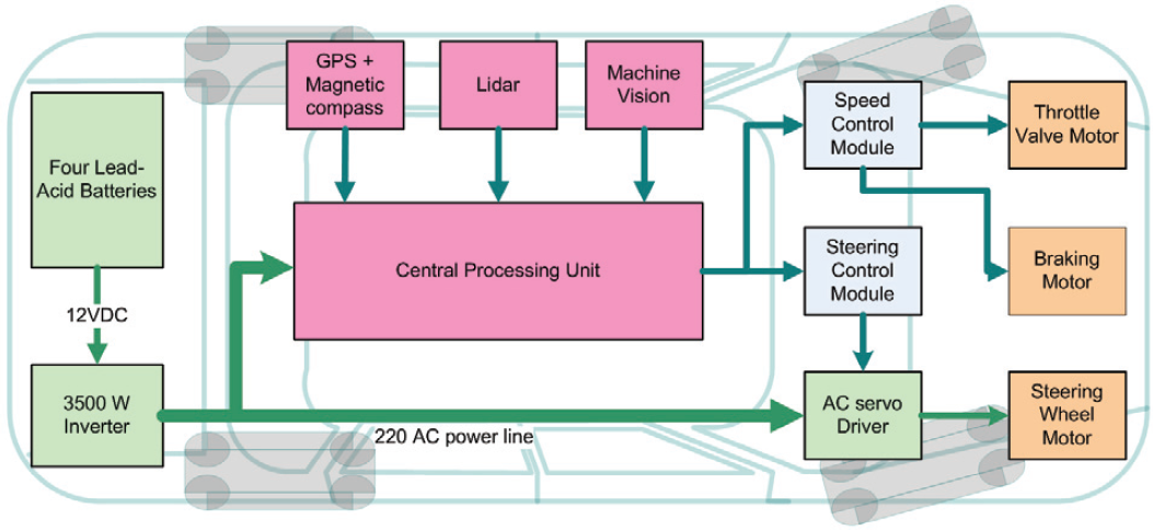
Overall architecture of the AIT intelligent vehicle

Fig. 3.

GPS card and a magnetic compass

Fig. 4.

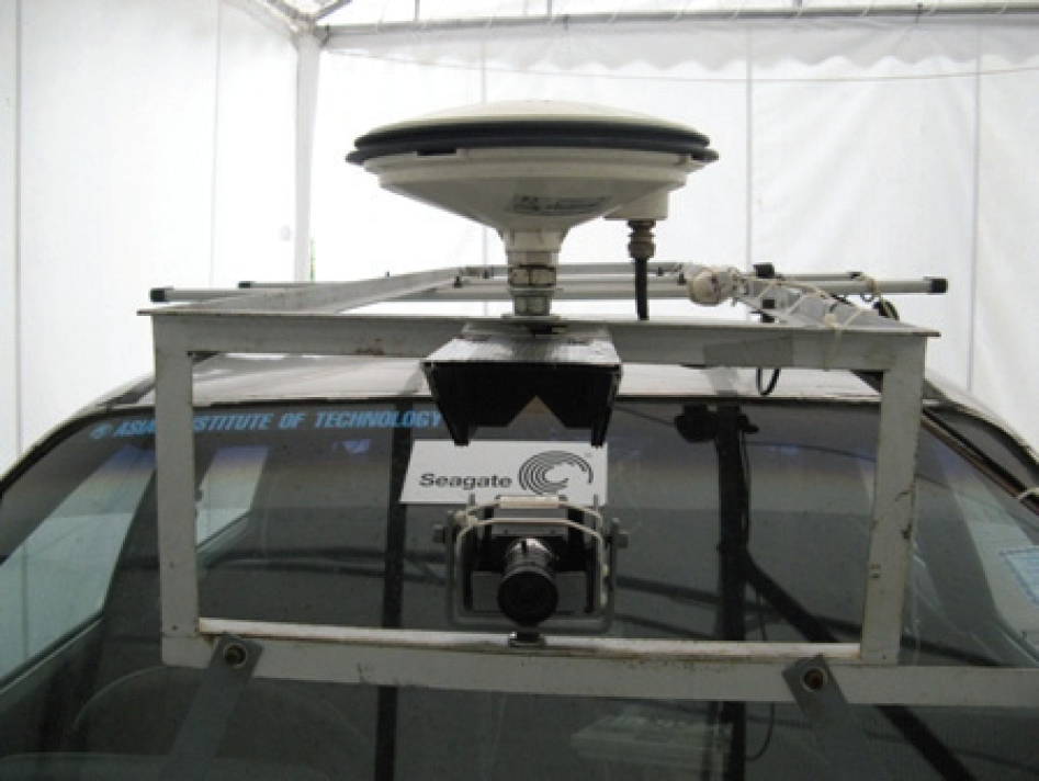
GPS antenna and a camera

3. Sensor Fusion Architecture

This section describes the sensor fusion algorithm based on the integration of a GPS, a magnetic compass and a camera, and the fuzzy number operations. Fig. 5 shows the sensor fusion flowchart.

Fig. 5.

Flowchart of the sensor fusion algorithm

3.1 Image processing

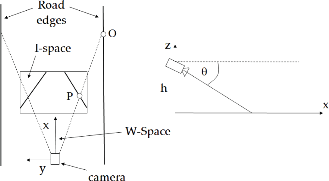
In the algorithm, two road images from two different waypoints are captured. Road center and road direction (θ _image ) are determined. One road image is used in determining horizontal error. The other road image is used in determining vertical error. Perspective distortion is solved by using inverse perspective mapping (IPM). Fig. 6 displays the relationship between the world coordinate (W-space) and the image coordinate (I-space). Point O in W-space corresponds to point P in I-space. Road edges, which are parallel in the world coordinate, become a vanishing point in the image coordinate. The position of the camera is defined as the center of W-space, using equation (1) and (2) (Bertozzi, M. et al, 1998).

$$u(x,y)=\frac{{\tan }^{-1}\left[\frac{h\sin \left({\tan }^{-1}\left(\frac{y}{x}\right)\right)}{y}\right]-(\theta -\alpha )}{\frac{2\alpha }{n-1}}$$

(1)

$$v(x,y)=\frac{{\tan }^{-1}\left(\frac{y}{x}\right)+\alpha }{\frac{2\alpha }{m-1}}$$

(2)

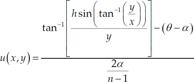
where h is the height of the camera above ground, θ is the angle between the optical axis and horizontal axis, 2α is the camera aperture, and n × m is the resolution of image.

Fig. 6.

Inverse perspective mapping

To identify the road segment in an image, hue and saturation thresholdings are utilized. Hue thresholding is basically used for thresholding road pixel without shadow. On the other hand, saturation thresholding plays an important role for thresholding road segment under shadow. These two thresholdings compliment each other very well to identify the road segment. In hue thresholding, reference hue value is computed by averaging hue values inside a 40 × 40 window at the center lowest part of the image before inverse perspective mapping. Based on the camera installation, most pixels inside this area are road pixels.

The pixels which have hue value within ±8 of the reference hue value are recognized as road pixels, white pixels, otherwise black pixels. For the road pixels under shadow, the saturation value is very low. In the algorithm, the pixels that have saturation value below 20 are also recognized as road pixels.

Because of non-smooth condition of the road, some noises deteriorate the road image. 5 × 5 median filter is used along with closing operation to remove these noises. Median filter cannot perfectly eliminate salt and pepper noises. Therefore, closing operation helps closing all small black blobs inside the road area.

Canny Edge Detector is applied to identify road edges. However, after edge detection, some noises exist in the image. In order to suppress these noises, thresholding based on the length of feature is applied. Features that are shorter than 200 pixels are eliminated. Next, two lines are drawn at the 150^th and the 180^th rows resulting in four intersecting points as shown in Fig. 7. In the first road image, two intersecting points on each row as center pixels $(x_1^1,y_1^1)$ and $(x_2^1,y_2^1)$ on the 150^th and the 180^th rows respectively. Similarly, $(x_1^2,y_1^2)$ and $(x_2^2,y_2^2)$ are the center pixels on the 150^th and the 180^th rows respectively in the second road image. Road direction is determined from

$${\theta }_{image}={\tan }^{-1}\left(\frac{x_2-x_1}{y_2-y_1}\right)$$

(3)

Fig. 7.

Road edges after Canny Edge Detector

3.2 Global vehicle position estimation

The pixel ( $(x_2^1,y_2^1)$ is the average position of the left and right road edges on the 180^th row. It is used as the local reference of the road center which is basically the waypoint for the vehicle to track. The absolute position of $(x_2^1,y_2^1)$ can be computed by translating the global current position of the vehicle by lateral and longitudinal offset in the road coordinate. Therefore, it is necessary to accurately estimate the exact current position of the vehicle. This initial position is determined by making the vehicle stay still and collecting its latitudes and longitudes. The histograms of both latitude and longitude are plotted. The mode values of the position from the histograms representing the current latitude and longitude of the vehicle are determined. These positions are denoted by $ugv\_av{g}_{lat}^{world}$ and $ugv\_av{g}_{lon}^{world}$ along with the uncertainties (δ _lat , δ _lon ) in the form of standard deviations. The more data is received, the more accurate position is achieved.

Since information from all the sensors contain some uncertainties, their output readings can be considered as fuzzy numbers. Alpha-cut of each fuzzy number is a closed interval of real number. Thus, arithmetic operations on fuzzy numbers can be determined by applying arithmetic operations on the closed interval as followings.

$$[a,b]+[c,d]=[a+c,b+d]$$

(4)

$$[a,b]-[c,d]=[a-c,b-d]$$

(5)

$$[a,b]\times [c,d]=[min(ac,ad,bc,bd),max(ac,ad,bc,bd)]$$

(6)

$$[a,b]/[c,d]=[min(\frac{a}{c},\frac{a}{d},\frac{b}{c},\frac{b}{d}),max(\frac{a}{c},\frac{a}{d},\frac{b}{c},\frac{b}{d})]$$

(7)

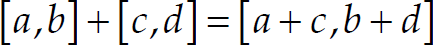
when 0 is not in [c, d]

In the algorithm, all the fuzzy numbers are modeled by triangular shape centered at the value read from the sensor with a base width of two times of the tolerance. Fig. 8 shows membership function of the vehicle longitude in the world coordinate.

Fig. 8.

Membership function of vehicle longitude in the world coordinate

The alpha-cut of the vehicle longitude can be expressed by

$$[{\delta }_{lon}(\mu -1)+ug{v}_{-}av{g}_{lon}^{world},ug{o}_{-}au{g}_{lon}^{world}-{\delta }_{lon}(\mu -1)]$$

(8)

Fig. 9 shows membership function of the vehicle latitude in the world coordinate.

Fig. 9.

Membership function of vehicle latitude in the world coordinate

The alpha-cut of the vehicle latitude can be expressed by

$$[{\delta }_{lat}(\mu -1)+ug{v}_{-}av{g}_{lat}^{world},ug{o}_{-}au{g}_{lat}^{world}-{\delta }_{lat}(\mu -1)]$$

(9)

3.3 Vehicle position in vehicle coordinate and road coordinate

Since the GPS provides information respect to the world coordinate but the camera provides information respect to the road coordinate, this two information must be converted to the same reference before integration. The world coordinate is firstly translated to the vehicle coordinate so that the current vehicle position locates at the origin point of the vehicle coordinate. Then, the vehicle coordinate is rotated using a rotational matrix to obtain the road coordinate. Fig. 10 shows these coordinate systems. The rotational matrix is characterized solely by rotational angle (θ _rotation ). This rotational angle is determined from the vehicle heading read from a magnetic compass and the road direction determined from a road image as shown in Fig. 11.

Fig. 10.

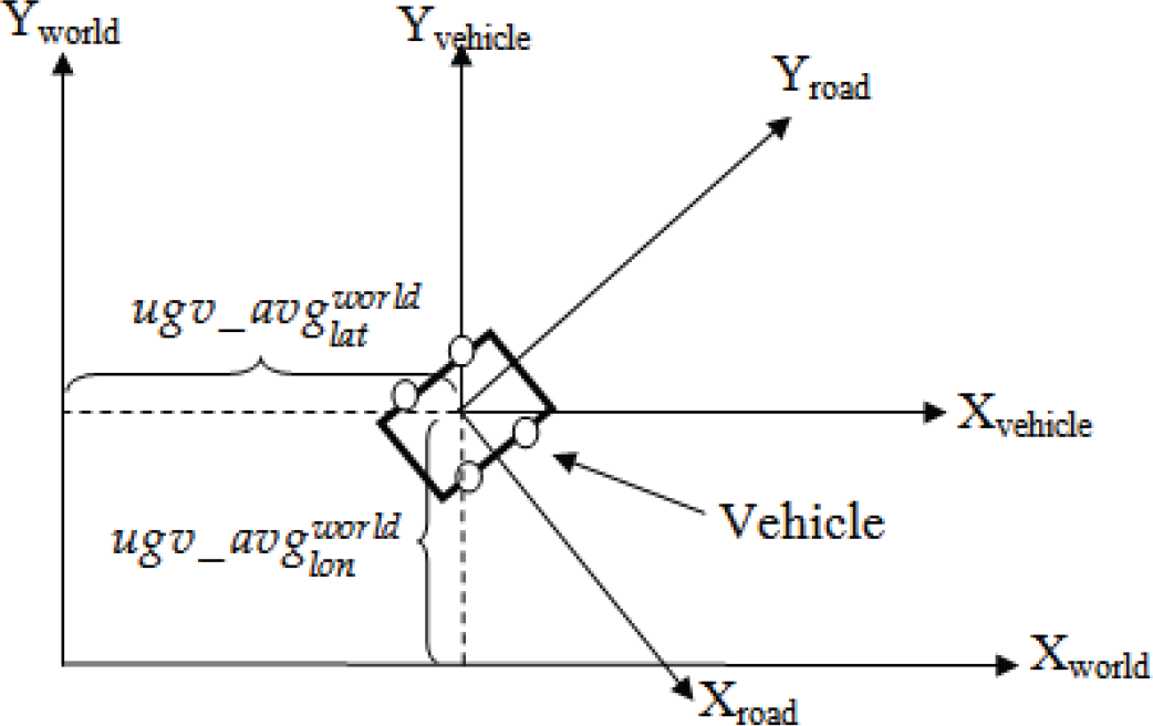
World, vehicle, and road coordinates

Fig. 11.

Vehicle heading and road direction

The vehicle heading is summed with the road direction θ _image according to equation (10) in order to obtain the rotational angle.

$${\theta }_{rotation}={\theta }_{image}+{\theta }_{compass}$$

(10)

To obtain θ _rotation within the first four quadrants, equation (11) is applied

$${\theta }_{rotation}=\{\begin{array}{ll}{\theta }_{rotation}-360& \text{when}{\theta }_{rotation}\ge 360\\ {\theta }_{rotation}& \text{when}{\theta }_{rotation}<360\end{array}$$

(11)

Fig. 12 shows membership function of the rotational angle. The alpha-cut of the rotational angle can be expressed by

$$[{\delta }_{\theta }(\mu -1)+{\theta }_{rotation},{\theta }_{rotation}-{\delta }_{\theta }(\mu -1)]$$

(12)

Fig. 12.

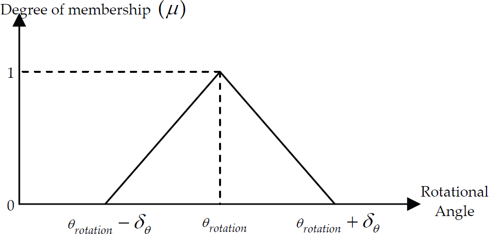
Membership function of rotational angle

After defining all fuzzy numbers, the vehicle longitude and latitude in the vehicle coordinate are then determined. This can be done by translating the world coordinate horizontally by $ugv\_av{g}_{lon}^{world}$ and vertically by $ugv\_av{g}_{lat}^{world}$ . The alpha-cuts of $ug{v}_{lon}^{vehicle}$ and $ug{v}_{lat}^{vehicle}$ , thus, become

$$[{\delta }_{lon}(\mu -1),-{\delta }_{lon}(\mu -1)]$$

(13)

$$[{\delta }_{lat}(\mu -1),-{\delta }_{lat}(\mu -1)]$$

(14)

Let's denote

$$lo{n}_l^1={\delta }_{lon}(\mu -1)$$

(15)

$$lo{n}_r^1={\delta }_{lon}(\mu -1)$$

(16)

$$la{t}_l^1={\delta }_{lon}(\mu -1)$$

(17)

$$la{t}_r^1={\delta }_{lon}(\mu -1)$$

(18)

After obtaining the rotational angle, latitude and longitude of the current position of the vehicle, the vehicle coordinate is converted to the road coordinate by vehicle-to-road rotational matrix as shown in equation (19).

$$\left[\begin{array}{c}ug{v}_{road}^{lon}\\ ug{o}_{road}^{lat}\end{array}\right]=\left[\begin{array}{cc}\cos {\theta }_{rotation}& -\sin {\theta }_{rotation}\\ \sin {\theta }_{rotation}& \cos {\theta }_{rotation}\end{array}\right]\left[\begin{array}{c}ug{v}_{lon}^{uehicle}\\ ug{v}_{lat}^{uehicle}\end{array}\right]$$

(19)

Since the rotational angle is associated with trigonometry functions used in the rotational matrix, the extension principle which relates a fuzzy set to other mathematical functions is applied. The alpha-cuts of cos θ _rotation and sin θ _rotation can be expressed by

$$[\cos ({\delta }_{\theta }(\mu -1)+{\theta }_1),\cos ({\theta }_1-{\delta }_{\theta }(\mu -1))]$$

(20)

$$[\sin ({\delta }_{\theta }(\mu -1)+{\theta }_1),\sin ({\theta }_1-{\delta }_{\theta }(\mu -1))]$$

(21)

Let's denote

$$c_1=\cos ({\delta }_{\theta }(\mu -1)+{\theta }_1)$$

(22)

$$c_2=\cos ({\theta }_1-{\delta }_{\theta }(\mu -1))$$

(23)

$$s_1=\sin ({\delta }_{\theta }(\mu -1)+{\theta }_1)$$

(24)

$$s_2=\sin ({\theta }_1-{\delta }_{\theta }(\mu -1))$$

(25)

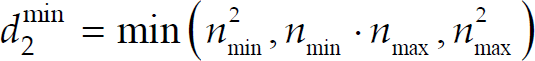
The next step is to find the current position of the vehicle in the road coordinate system. According to equation (19), to obtain the alpha-cut of $ug{v}_{lon}^{road}$ , the alpha-cuts of $ug{v}_{lon}^{vehicle}\cdot cos{\theta }_{retation}$ and $ug{v}_{lat}^{vehicle}\cdot sin{\theta }_{retation}$ must be firstly determined.

$$[min(lo{n}_l^1{c}_1,lo{n}_r^1{c}_2,lo{n}_r^1,lo{n}_r^1{c}_2),max(lo{n}_l^1{c}_1,lo{n}_l^1{c}_2,lo{n}_l^1{c}_1,lo{n}_r^1{c}_2)]$$

(26)

$$[min(la{t}_l^1{s}_1,la{t}_r^1{s}_2,la{t}_r^1{s}_1,la{t}_r^1{s}_2),max(la{t}_l^1{s}_1,la{t}_l^1{s}_2,la{t}_l^1{s}_1,la{t}_r^1{s}_2)]$$

(27)

Let's denote

$$lo{n}_c^{min}=min(lo{n}_l^1{c}_1,lo{n}_l^1{c}_2,lo{n}_r^1{c}_1,lo{n}_r^1{c}_2)$$

(28)

$$lo{n}_c^{max}=max(lo{n}_l^1{c}_1,lo{n}_l^1{c}_2,lo{n}_r^1{c}_1,lo{n}_r^1{c}_2)$$

(29)

$$la{t}_s^{min}=min(la{t}_l^1{s}_1,la{t}_l^1{s}_2,la{t}_r^1{s}_1,la{t}_r^1{s}_2)$$

(30)

$$la{t}_s^{max}=max(la{t}_l^1{s}_1,la{t}_l^1{s}_2,la{t}_r^1{s}_1,la{t}_r^1{s}_2)$$

(31)

By using the property of the closed interval subtraction, the alpha-cut of $ug{v}_{lon}^{road}$ results in

$$[lo{n}_c^{min}-la{t}_s^{max},lo{n}_c^{max}-la{t}_s^{min}]$$

(32)

Similarly, the alpha-cut of $ug{v}_{lat}^{road}$ can be computed in the same way. Firstly, alpha-cuts of $ug{v}_{lon}^{vehicle}\cdot sin{\theta }_{rotation}$ and $ug{v}_{lat}^{vehicle}\cdot cos{\theta }_{rotation}$ are determined.

$$[min(lo{n}_l^1{s}_1,lo{n}_l^1{s}_2,lo{n}_r^1{s}_1,lo{n}_r^1{s}_2),max(lo{n}_l^1{s}_1,lo{n}_l^1{s}_2,lo{n}_r^1{s}_1,lo{n}_r^1{s}_2)]$$

(33)

$$[min(la{t}_l^1{c}_1,la{t}_l^1{c}_2,la{t}_r^1{c}_1,la{t}_r^1{c}_2),max(la{t}_l^1{c}_1,la{t}_l^1{c}_2,la{t}_r^1{c}_1,la{t}_r^1{c}_2)]$$

(34)

Let's denote

$$lo{n}_s^{min}=min(lo{n}_l^1{s}_1,lo{n}_l^1{s}_2,lo{n}_r^1{s}_1,lo{n}_r^1{s}_2)$$

(35)

$$lo{n}_s^{max}=max(lo{n}_l^1{s}_1,lo{n}_l^1{s}_2,lo{n}_r^1{s}_1,lo{n}_r^1{s}_2)$$

(36)

$$la{t}_c^{min}=min(la{t}_l^1{c}_1,la{t}_l^1{c}_2,la{t}_r^1{c}_1,la{t}_r^1{c}_2)$$

(37)

$$la{t}_c^{max}=max(la{t}_l^1{c}_1,la{t}_l^1{c}_2,la{t}_r^1{c}_1,la{t}_r^1{c}_2)$$

(38)

Then, by using the property of the closed interval addition, the alpha-cut of $ug{v}_{lat}^{road}$ results in

$$[lo{n}_s^{min}+la{t}_c^{min},lo{n}_s^{max}+la{t}_c^{max}]$$

(39)

3.4 Lateral and longitudinal offsets

From Fig. 13, the global position of the selected pixel $(x_2,y_2^1)$ can be determined by translating the current local position of the vehicle $(ug{v}_{lon}^{road},ug{v}_{lat}^{raod})$ along x-axis by lateral offset and y-axis by longitudinal offset in the road coordinate. The longitudinal offset is fixed since the chosen row on the road image is fixed. It is selected at 2.5 m in front of the vehicle. On the other hand, the lateral offset is selected to be the length between x₂ and the center column, the 160^th column, of the road image. This deviation represents the distance from the center of the vehicle to the road center in pixel unit. The lateral offset is then converted to meter unit similar to the longitudinal offset.

Fig. 13.

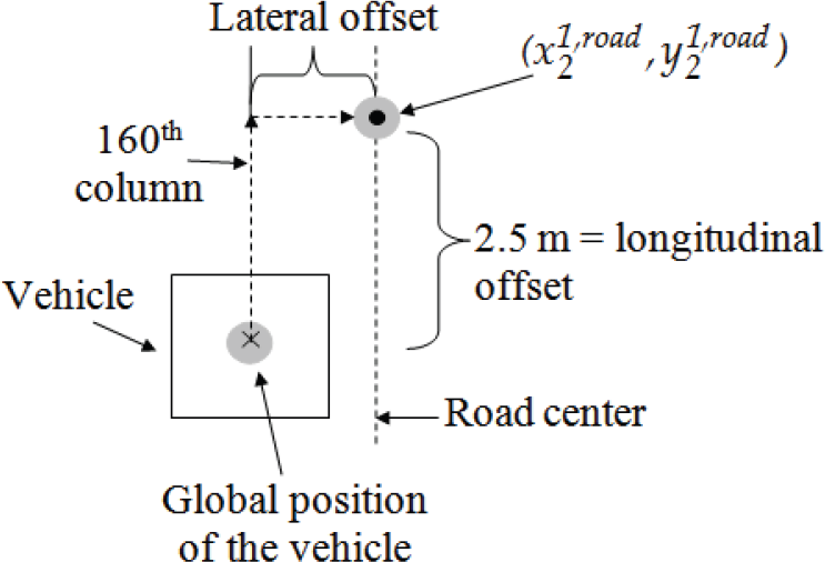
Lateral and longitudinal offsets

A calibration experiment is conducted to acquire the relationship between distance in pixel and distance in meter of the road image at 2.5 m in front of the vehicle. The camera on the vehicle captures images containing different objects at known length in meter. The distances are then counted in pixel length. The results are plotted as shown in Fig. 14. A straight line is fitted. The maximum error of this data is expressed as δ _pixel . The relationship between distance in meter and distance in pixel is expressed in equation (40).

$$\text{distance in meter}=0.0672\times \text{distance in pixel}$$

(40)

Fig. 14.

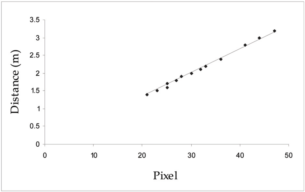
Relationship between distance in pixel and distance in meter

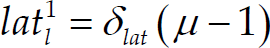
As a result, the lateral offset can be calculated by the following equation

$$\text{lateral offset}=d_m=0.0672\times (160-x_2^1)$$

(41)

Fig. 15 shows membership function of the lateral offset. The alpha-cut of the lateral offset can be expressed by

$$[({\delta }_{pixel}(\mu -1)+d_m),(d_m-{\delta }_{pixel}(\mu -1))]$$

(42)

Fig. 15.

Membership function of lateral offset

Let's denote

$$d_1^{min}={\delta }_{pixel}(\mu -1)+d_m$$

(43)

$$d_1^{min}=d_m-{\delta }_{pixel}(\mu -1)$$

(44)

3.5 Selected pixel position in road coordinate and vehicle coordinate

To obtain the global position of the selected pixel $\left(x_2^{1,road},y_2^{1,road}\right)$ , the following equations are applied.

$$x_2^{1,road}=ug{v}_{lon}^{road}+\frac{\text{lateral offset}}{\text{EM\_Scale}}$$

(45)

$$y_2^{1,road}=ug{v}_{lat}^{road}+\frac{2.5}{\text{NS\_Scale}}$$

(46)

where EW_Scale = 106080 m/degree and NS_Scale = 109369.2 m/degree. These two parameters are used in unit conversion of latitude and longitude from degree to meter.

The alpha-cuts of both $x_2^{1,road}$ and $y_2^{1,road}$ are

$$[lo{n}_c^{min}-la{t}_s^{max}+\frac{d_1^{min}}{E{W}_{-}Scale},lo{n}_c^{max}-la{t}_s^{min}+\frac{d_1^{max}}{E{W}_{-}Scale}]$$

(47)

$$[lo{n}_s^{min}-la{t}_c^{max}+\frac{2.5}{N{S}_{-}Scale},lo{n}_s^{max}-la{t}_c^{min}+\frac{2.5}{E{W}_{-}Scale}]$$

(48)

Let's denote

$$x_{2,rd}^{1,min}=lo{n}_c^{min}-la{t}_s^{max}+\frac{d_1^{min}}{E{W}_{-}Scale}$$

(49)

$$x_{2,rd}^{1,max}=lo{n}_c^{max}-la{t}_s^{max}+\frac{d_1^{max}}{E{W}_{-}Scale}$$

(50)

$$y_{2,rd}^{1,min}=lo{n}_{min}^s+la{t}_{min}^c+\frac{2.5}{N{S}_{-}Scale}$$

(51)

$$y_{2,rd}^{1,max}=lo{n}_{max}^s+la{t}_{max}^c+\frac{2.5}{N{S}_{-}Scale}$$

(52)

3.6 Xoffset and yoffset determination

Fig. 16 shows x _offset and y _offset in road coordinate. Let's consider the road coordinate. When the line connecting the two waypoints of the first image aligns with the North Pole, x _offset is calculated by

$$x_{offset}=d_x\cdot \sin {\theta }_1$$

(53)

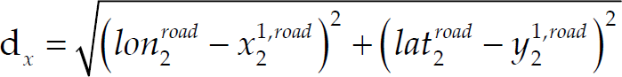
where d _x is the distance from the vehicle to the next waypoint. θ₁ is the angle from the vehicle to the next waypoint respect to the North Pole. d _x is computed from

$${\mathrm{d}}_x=\sqrt{{(lo{n}_2^{road}-x_2^{1,road})}^2+{(la{t}_2^{road}-y_2^{1,road})}^2}$$

(54)

Fig. 16.

x _offset and y _offset

The alpha-cuts of $\left(lo{n}_2^{road}-x_2^{1,road}\right)$ and $\left(la{t}_2^{road}-y_2^{1,road}\right)$ are

$$[lo{n}_{2,min}^{road}-x_{2,rd}^{1,max},lo{n}_{2,max}^{road}-x_{2,rd}^{1,min}]$$

(55)

$$[la{t}_{2,min}^{road}-y_{2,rd}^{1,max},la{t}_{2,max}^{road}-y_{2,rd}^{1,min}]$$

(56)

Let's denote

$$n_{min}=lo{n}_{2,min}^{road}-x_{2,rd}^{1,max}$$

(57)

$$n_{max}=lo{n}_{2,max}^{road}-x_{2,rd}^{1,min}$$

(58)

$$m_{min}=la{t}_{2,max}^{road}-y_{2,rd}^{1,max}$$

(59)

$$m_{max}=la{t}_{2,max}^{road}-y_{2,rd}^{1,min}$$

(60)

The alpha-cuts of ${\left(lo{n}_2^{road}-x_2^{1,road}\right)}^2$ and ${\left(la{t}_2^{road}-y_2^{1,road}\right)}^2$ are

$$[min(n_{min}^2,n_{min}\cdot n_{max},n_{max}^2),max(n_{min}^2,n_{min}\cdot n_{max},n_{max}^2)]$$

(61)

$$[min(m_{min}^2,m_{min}\cdot m_{max},m_{max}^2),max(m_{min}^2,m_{min}\cdot m_{max},m_{max}^2)]$$

(62)

Let's denote

$$d_2^{min}=min(n_{min}^2,n_{min}\cdot n_{max},n_{max}^2)$$

(63)

$$d_2^{max}=max(n_{min}^2,n_{min}\cdot n_{max},n_{max}^2)$$

(64)

$$d_3^{min}=min(m_{min}^2,m_{min}\cdot m_{max},m_{max}^2)$$

(65)

$$d_3^{max}=max(m_{min}^2,m_{min}\cdot m_{max},m_{max}^2)$$

(66)

The alpha-cut of d _x becomes

$$[\sqrt{d_2^{min}+d_3^{min}},\sqrt{d_2^{max}+d_3^{max}}]$$

(67)

Let's denote

$$d_x^{min}\sqrt{d_2^{min}+d_3^{min}}$$

(68)

$$d_x^{max}\sqrt{d_2^{max}+d_3^{max}}$$

(69)

The alpha-cut of x _offset can be expressed by

$$\begin{gathered} [min(d_x^{min}\cdot \sin {\theta }_1^{min},d_x^{min}\cdot \sin {\theta }_1^{max},d_x^{max}\cdot \sin {\theta }_1^{min},d_x^{max}\cdot \sin {\theta }_1^{max}), \\ max(d_x^{min}\cdot \sin {\theta }_1^{min},d_x^{min}\cdot \sin {\theta }_1^{max},d_x^{max},\cdot \sin {\theta }_1^{min},d_x^{max}\cdot \sin {\theta }_1^{max})] \end{gathered}$$

(70)

y _offset is calculated by the following equation.

$$y_{offset}=\{\begin{array}{l}\frac{-d_y}{\sin {\theta }_{23}}\cdot \sin {\theta }_3\text{if}0<{\theta }_2<90\text{and}180<{\theta }_2<270\\ \frac{d_y}{\sin {\theta }_{23}}\cdot \sin {\theta }_3\text{if}90<{\theta }_2<180\text{and}270<{\theta }_2<360\end{array}$$

(71)

where d _y is the distance from the vehicle to the next waypoint in the second image. θ₂₃ is the direction of the line connecting the two waypoints respect to the North Pole. θ₂ is the heading from the vehicle to the next waypoint respectively. The alpha-cut of $\frac{d_y}{sin{\theta }_{23}}$ is expressed by

$$\begin{gathered} \begin{array}{r}[min(\frac{d_y^{min}}{\sin {\theta }_{23}^{min}},\frac{d_y^{min}}{\sin {\theta }_{23}^{max}},\frac{d_y^{max}}{\sin {\theta }_{23}^{min}},\frac{d_y^{max}}{\sin {\theta }_{23}^{max}}), \\ max(\frac{d_y^{min}}{\sin {\theta }_{23}^{min}},\frac{d_y^{min}}{\sin {\theta }_{23}^{max}},\frac{d_y^{max}}{\sin {\theta }_{23}^{min}},\frac{d_y^{max}}{\sin {\theta }_{23}^{max}})]\end{array} \end{gathered}$$

(72)

Let's denote

$$d_{y,\sin }^{min}=min(\frac{d_y^{min}}{\sin {\theta }_{23}^{min}},\frac{d_y^{min}}{\sin {\theta }_{23}^{max}},\frac{d_y^{max}}{\sin {\theta }_{23}^{min}},\frac{d_y^{max}}{\sin {\theta }_{23}^{max}})d_{y,\sin }^{min}=min(\frac{d_y^{min}}{\sin {\theta }_{23}^{min}},\frac{d_y^{min}}{\sin {\theta }_{23}^{max}},\frac{d_y^{max}}{\sin {\theta }_{23}^{min}},\frac{d_y^{max}}{\sin {\theta }_{23}^{max}})$$

(73)

$$d_{y,\sin }^{max}=max(\frac{d_y^{min}}{\sin {\theta }_{23}^{min}},\frac{d_y^{min}}{\sin {\theta }_{23}^{max}},\frac{d_y^{max}}{\sin {\theta }_{23}^{min}},\frac{d_y^{max}}{\sin {\theta }_{23}^{max}})$$

(74)

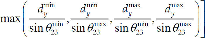
Hence, the alpha-cut of y _offset becomes

$$\begin{array}{r}[min(d_{y,\sin }^{min}\cdot \sin {\theta }_3^{min},d_{y,\sin }^{min}\cdot \sin {\theta }_3^{max},d_{y,\sin }^{max}\cdot \sin {\theta }_3^{max},d_{y,\sin }^{max}\cdot \sin {\theta }_3^{max}),\\ max(d_{y,\sin }^{min}\cdot \sin {\theta }_3^{min},d_{y,\sin }^{min}\cdot \sin {\theta }_3^{max},d_{y,\sin }^{max}\cdot \sin {\theta }_3^{min},d_{y,\sin }^{max}\cdot \sin {\theta }_3^{max})]\end{array}$$

(75)

4. Experimental Result

4.1 Result on map error correction

The experiment is conducted on an unmarked road inside AIT campus. The image of a course track acquired from Google Earth is shown in Fig. 17. The white line drawn in the Google Earth map shows the path that the vehicle has to follow. There are 12 waypoints in the experiment as shown in Table 1. If these waypoints are provided directly to the vehicle, the vehicle will run out of the road. This problem is resulted from position error of the Google Earth map.

Fig. 17.

Course track

Table 1.

Latitude and longitude of original map

Waypoint #	Latitude	Longitude
1	14.081724	100.610726
2	14.082292	100.610737
3	14.082825	100.610746
4	14.083090	100.610742
5	14.083274	100.610712
6	14.083385	100.610699
7	14.083440	100.610727
8	14.083482	100.610789
9	14.083521	100.610903
10	14.083513	100.611848
11	14.083478	100.611923
12	14.083404	100.611959

The camera is equipped at the center of the vehicle and 1.35 m above the ground on the front windshield. The image is resized from 480 × 640 to 240 × 320 in order to reduce the processing time. Thus, the 160^th column represents the center position of the image and the vehicle. The images are converted from RGB to gray scale. The result of the inverse perspective mapping is shown in Table 2.

Table 2.

Comparison of images before and after IPM

After hue and saturation thresholding, the image is displayed in black and white pixels as shown in Fig. 18. After Canny Edge Detector and length of contour thresholding, the small white noises on the right hand side in Fig. 18 are eliminated resulting in the image shown in Fig. 19.

Fig. 18.

Result of hue and saturation thresholding

Fig. 19.

Road edges result

Table 3 shows locations of the left and the right edges on the 150^th and the 180^th rows and the center position on both rows and also the road direction.

Table 3.

Comparison of images before and after IPM

	Left edge	Right edge	Center edge
150th row	136	172	154
180th row	134	170	152
Road direction		3.814 degree

Fig. 20 shows 200 data of the latitudes and longitudes from the GPS.

Fig. 20.

Latitude and longitude for vehicle current position estimation

The results from the experiment show that the first global vehicle position is

$$\begin{array}{r}ug{o}_{-}au{g}_{lat}^{world}=14.08189218\text{degree}{\delta }_{lat}=0.141859344\mathrm{m}\\ ug{o}_{-}av{g}_{lon}^{world}=100.6106577\text{degree}{\delta }_{lon}=0.243895656\mathrm{m}\end{array}$$

And the second global vehicle position is

$$\begin{array}{r}ug{o}_{-}au{g}_{lat}^{world}=14.08350902\text{degree}{\delta }_{lat}=0.211237645\mathrm{m}\\ ug{o}_{-}av{g}_{lon}^{world}=100.6111889\text{degree}{\delta }_{lon}=0.253438574\mathrm{m}\end{array}$$

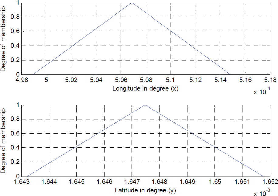
Based on these data, membership functions of longitude and latitude of the first and the second vehicle position in the world coordinate are expressed in Fig. 21 and Fig. 22 respectively.

Fig. 21.

Membership functions of longitude and latitude of the first vehicle position in the world coordinate

Fig. 22.

Membership functions of longitude and latitude of the second vehicle position in the world coordinate

The initial heading read from the magnetic compass is 358.2°. On the other hand, θ _image is 3.814°. Thus, the rotational angle is 2.014°. The result of rotational angle membership function is shown in Fig. 23.

Fig. 23.

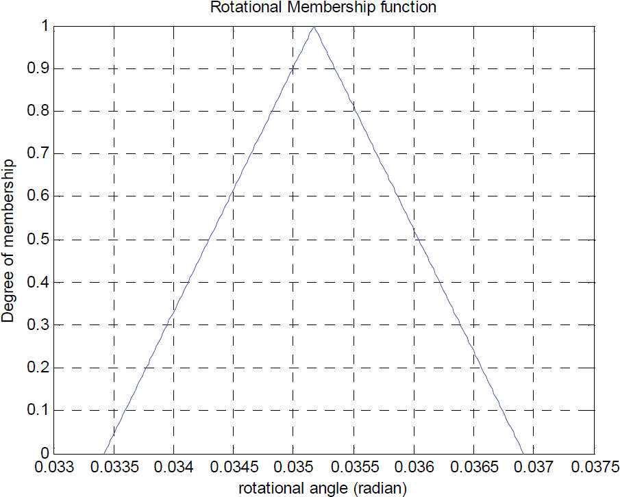
Membership function of rotational angle

By using the extension principle, cosθ _rotation and sinθ _rotation can be expressed in terms of fuzzy numbers as well. The results of cosine and sine membership functions are shown in Fig. 24.

Fig. 24.

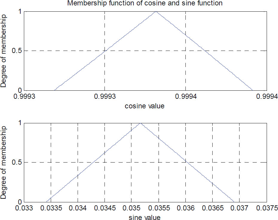
Membership functions of cosine and sine functions

In fact, the shapes of membership functions of cosθ _rotation and sinθ _rotation are not triangle. The membership functions are the results from very small angular uncertainty, around 0.1°. Thus, cosine and sine functions are taken only on small interval of rotational angle. However, if the uncertainty is larger, the membership functions will deviate from triangular shape. Fig. 25 illustrates the membership functions of cosθ _rotation and sinθ _rotation when rotational angle is 2.014° with uncertainty of 5°.

Fig. 25.

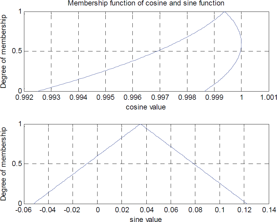
Membership functions of cosine and sine functions when rotational angle is 2.014° and its uncertainty is 5°.

After obtaining the position of the vehicle in the road coordinate, the membership functions of $x_2^{1,road}$ and $y_2^{1,road}$ are determined. The results are shown in Fig. 26.

Fig. 26.

Membership functions of x₂^1,road and y₂^1,road

Fig. 27 shows the membership functions of $(x_2^{2,road},y_2^{2,road})$ which is the longitude and latitude of the second global vehicle position in the road coordinate system.

Fig. 27.

Membership functions of x₂^2,road and y₂^2,road

The membership functions of x _offset and y _offset are shown in Fig. 28.

Fig. 28.

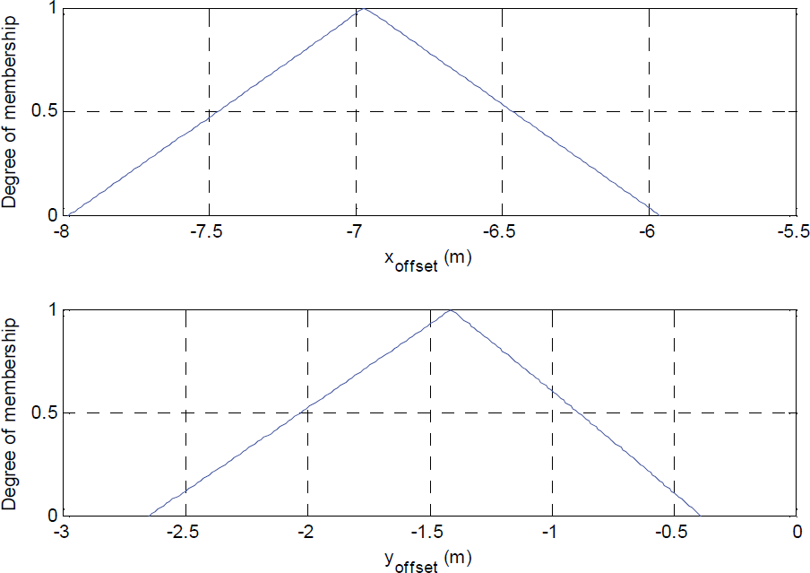
Membership functions of x _offset and y _offset

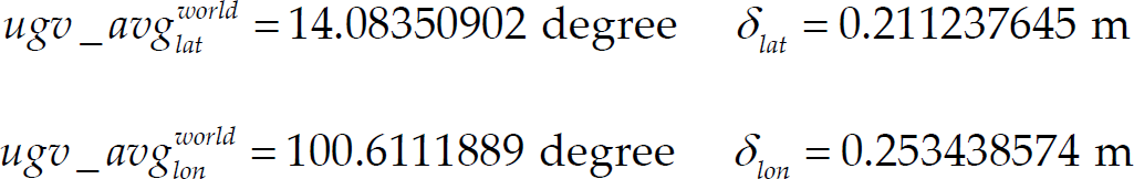
According to Fig. 28, x _offset and y _offset have the highest degree of membership at

$$\begin{array}{r}{x}_{offset}=-6.978\mathrm{m}\\ y_{offset}=-1.414\mathrm{m}\end{array}$$

By using these x _offset and y _offset , the new waypoints are generated. The result is shown in Fig. 29. The light color line is the original waypoints. The dark color line is the new map which is shifted horizontally to the left by 6.978 m and vertically downward by 1.414 m.

Fig. 29.

New waypoints versus old waypoints

4.2 Result on vehicle control

After correcting the waypoints, they are provided to the vehicle control system. This control system is designed based on fuzzy logic controller with two inputs and one output. The first input is the lateral offset from the vehicle to the line connecting the previous and next waypoint. The other input is the heading error which is the angle difference between the vehicle heading direction and the direction from the previous waypoint to the next waypoint. The output is the steering angle. All membership functions of the inputs and the output are modeled as triangular shape as shown in Fig. 30 (a), (b), and (c). Fuzzy inference rules are designed and shown in Table 4.

Fig. 30.

Membership functions of the heading error input (a), lateral offset input (b), and the steering angle output (c)

Table 4.

Fuzzy inference rules

		Heading error
		LN	N	0	P	LP
Lateral offset	LN	FR	FR	MR	0	ML
	N	FR	MR	SR	SL	ML
	0	MR	SR	0	SL	ML
	P	MR	SR	SL	ML	FL
	LP	MR	0	ML	FL	FL

Fig. 31 shows the result of vehicle latitudes and longitudes during autonomous running along with the original and the corrected waypoints. The result shows that the AIT intelligent vehicle successfully tracked the road center.

Fig. 31.

The actual positions of the vehicle compared to the old and new waypoints.

Where

LN = large negative

N = negative

SL = small left

ML = medium left

FL = fully left

LP = large positive

P = positive

SR = small right

MR = medium right

FR = fully right

5. Conclusion

This paper described an algorithm used to correct inaccuracy of the available maps such as Google Earth. The proposed algorithm corrected and compensated the error by using fuzzy based sensor fusion concept. Three sensor devices, a GPS, a magnetic compass and a camera, were integrated in order to determine the offset that the original waypoints were away from the road center in both horizontal and vertical directions. Furthermore, all arithmetic operations were conducted based on the alpha-cut closed interval arithmetic so that the uncertainties of the sensors were also taken into account. After knowing the horizontal and vertical offsets, the initial path was shifted accordingly. This algorithm performed very well in the experiment. The proposed algorithm was very easy to implement, low cost and less time consuming compared to other commonly used methods such as driving and collecting waypoints or assuming that all the given waypoints were accurate.