Sage Journals: Discover world-class research

Abstract

General purpose visual programming languages (VPLs) promote the construction of programs that are more comprehensible, robust, and maintainable by enabling programmers to directly observe and manipulate algorithms and data. However, they usually do not exploit the visual representation of entities in the problem domain, even if those entities and their interactions have obvious visual representations, as is the case in the robot control domain. We present a formal control model for autonomous robots, based on subsumption, and use it as the basis for a VPL in which reactive behaviour is programmed via interactions with a simulation.

Keywords

visual programming direct manipulation demonstration subsumption reactive behaviour

1. Introduction

Many problem domains consist of entities that have commonly accepted visual representations. An example in the realm of software application development, is graphical user interfaces (GUIs), which were originally programmed by writing code in standard textual programming languages. Because interface elements have standardised, well understood visual representations and behaviours, an obvious step was to create tools with which GUIs could be built by directly assembling interface elements, and even programming some of their interactions and behaviours by demonstration (B. & Buxton, W. (1986): Wolber, D. (1997)), or drawing various kinds of connecting lines (Carrel-Billiard, M. & Akerley, J. (1998)). GUIs are now almost exclusively built using such direct-manipulation tools.

Another such ‘concrete’ domain, populated with entities with obvious visual representations and observable behaviours, is robot programming. A robot control program consists of algorithms built on the primitive actions the robot can perform, at least some of which are physically observable, such as changes in position or colour, grasping, pushing and so forth. Just as the concreteness of GUIs led to the development of GUI builders, the concreteness of the robot world has motivated researchers and practitioners to search for ways to program robots by direct manipulation. A simple application of this idea is the training of industrial robots to perform repetitive tasks in a completely known environment by simply recording the actions of an experienced operator doing the task, painting car panels on an assembly line for example. In recent years, many aspects of this promising paradigm have received close attention (Billard, A. & Dillmann, R. (2004): Billard, A. & Siegwart, R. (2004)), such as training a robot by interacting with a simulation rather than with the actual robot (Aleotti, J.; Caselli, S. & Reggiani, M. (2004)), improving task performance through practice (Bentivegna, D.C.; Atkeson C.G. & Cheng, G. (2004)), and optimisation of imitative learning (Billard, A.; Epars, Y.; Calinon, S.; Schaal S. & Cheng, G. (2004): Chella, A.; Dindo, H. & Infantino, I. (2006)).

Programming by Demonstration (pbd) is viewed by many as an elegant way to create behaviour by directly manipulating domain entities, as in the worlds of graphical user interfaces and robots (Cypher, A. (Ed.) (1993)). pbd entails the use of examples to teach an agent how to behave in situations analogous to those of the examples. A pbd system records the actions of the trainer and constructs a control program to govern the behaviour of the agent. Frequently, generalisation plays a part in this construction. Some systems infer more general rules of behaviour from the examples provided (St. Amant, R.; Lieberman, H.; Potter, R. & Zettlemoyer, L. (2000): Lau, T. (2001): Myers, B. & McDaniel, R. (2001)). Some provide the user with tools to manually generalise examples (Kahn, K. (2000): Michail, A. (1998)). In others, because of the nature of the underlying model, a rule generated from an example applies to a class of similar situations (Smith, D.C.; Cypher, A. & Spohrer, J. (1994)). The applicability of pbd to many problem domains has been examined (St. Amant, R.; Lieberman, H.; Potter, R. & Zettlemoyer, L. (2000): Lieberman, H.; Nardi, B. & Wright, D. (1999): Smith, D.C.; Cypher, A. & Spohrer, J. (1994)). For example, substantial work has been done on developing animated and cartoon-like programming environments to increase children's interest in programming, or to provide them with simple, interactive yet powerful educational tools (Gindling, J.; Ionnidou, A.; Loh, J.; Lokkebo O. & Repenning, A. (1995): Kahn, K. (2000): Repenning, A. (1995): Smith, D.C.; Cypher, A. & Spohrer, J. (1994)). Although pbd can be applied to domains in which the concepts are abstract (Lieberman, H. (1993)), it seems to have a natural fit with problems of a more concrete nature, as illustrated above. This notion of “concreteness” is also one of the main principles behind visual programming languages (VPLs). It was named “closeness of mapping” by Green and Petre (), who observed that the more directly a language represents entities, structures and interactions of the problem domain, the more useful, productive or efficient the language will be. Various studies support this observation. For example, a survey by Whitley and Blackwell of users of LabVIEW, a language for engineers in which control programs are represented as wiring diagrams (Johnson, G.W. (2006)), provides evidence that LabVIEW's close mapping between program and problem is advantageous (Whitley, K.N. & Blackwell, A.F. (2001)).

Robot programming has recently caught the attention of VPL researchers, prompted in part by a competition at the 1997 IEEE Symposium on Visual Languages, involving the application of VPLs to mobile robot programming (Ambler, A.L.; Green, T.; Kimura, T.D.; Repenning A. & Smedley, T.J. (1997)), and inspired by an example of programming a robot car using the rule-based mechanism of AgentSheets (Gindling, J.; Ionnidou, A.; Loh, J.; Lokkebo O. & Repenning, A. (1995)). Some examples giving the flavour of the approaches taken are as follows.

Altaira (Pfeiffer, J.J. (1997)) and Isaac (Pfeiffer, J.J. (1999)) both implement rule-based models for robot control, relying respectively on a variant of Brooks' subsumption model for robot control (Brooks, R.A. (1986)), and a fuzzy deductive system for geometric reasoning. Cocoa (Smith, D.C.; Cypher, A. & Spohrer, J. (1994)) also implements a rule-based model, and although not specifically designed for robot control, with minor changes it can be used for programming simple robots in a 2D environment. vbbl (Cox, P.T.; Risley, C.C. & Smedley, T.J. (1998)) is a message flow, domain-specific visual language based on subsumption, and designed as an extension to the application framework of Prograph CPX (Steinman, S.B. & Carver, K.G. (1995)). Altaira, Isaac and Cocoa allow representations of the robot to be included, but in all three, the coding of rules is a tedious task in which the robot representations play a rather minor role. vbbl, on the other hand is very general, but does not exploit any of the features of the robot. None of these incorporate the direct manipulation that is the cornerstone of pbd systems.

In (Cox, P.T. & Smedley, T.J. (1998)) it is noted that if a visual pbd language for robots were to exploit the features of the robot and environment by incorporating visual representations of them, then such a language would necessarily be limited to a specific robot in an environment composed of specific objects. In an attempt to reconcile concreteness with generality, a robot programming system was proposed consisting of two modules. The first part, the Hardware Definition Module (hdm), is a design environment in which a robot and other objects are modelled. The second part, the Software Definition Module (sdm), uses a description produced by hdm to present an environment in which the user programs a control system by manipulating a simulation of the robot. A structure for hdm was described in some detail, but sdm was addressed only superficially. Subsequently, Banyasad further developed the sdm concept (Banyasad, O. (2000)), based on a rather more structured version of Brooks' subsumption. A prototype programming environment was built, partly based on the latter proposal (Banyasad, O.; Cox, P.T. & Young, J. (2000)). Experiences with this prototype led to the significant refinement of the control model and improvement of the interface proposed in (Banyasad, O. (2000)), reported here.

In the following we provide a formal, subsumption-based definition for a control model for autonomous robots, suitable for the kind of visual programming-by-demonstration suggested in (Cox, P.T. & Smedley, T.J. (1998)), followed by a proposal for sdm, presented via an extended example.

2. Robots and control models

A robot is a programmable machine equipped with at least one actuator and at least one sensor. An actuator is a device that can release non-mechanical energy in its surrounding environment, such as light or other electromagnetic waves, or can mechanically change its environment, including itself. A sensor is a device that can detect or measure a specific kind of energy in its operating domain, for example, an infrared sensor, or a touch sensor. The sensors and actuators of a robot are connected by some structural parts collectively called the body, which has no significance for control or programming purposes except for the geometric relationships it imposes on sensors and actuators. Such robots are intended to operate in an environment which is at least partly unknown, in such a way that they can react sensibly when they encounter objects or otherwise detect changes. We are not, therefore, interested in robots that perform fully defined, repetitive tasks in a completely known environment such as an assembly line. Programs controlling robots must compute values for actuators based on the values of sensors. A robot's level of autonomy is the degree to which it can respond to environmental changes in a logical fashion as if it were being controlled by an operator. Examples of mobile autonomous robots are the Mars Rover (NASA Jet Propulsion Laboratory (2007): St. Amant, R.; Lieberman, H.; Potter, R. & Zettlemoyer, L. (2000)), autonomous underwater vehicles (Jackson, E. & Eddy, D. (1999): (1992)) and mobile office assistants (Simmons, R.; Goodwin, R.; Haigh, K.Z.; Koenig S. & O'Sullivan, J. (1997)).

Of the many control models for programming robots, the subsumption architecture due to Brooks is among the simpler ones. Since the control model we propose is based on this architecture, we give an overview of it below. A thorough discussion can be found elsewhere (Brooks, R.A. (1986)).

2.1. Brooks' Subsumption Architecture

The traditional method for designing a control system for a robot is to decompose the problem of computing actuator values from sensor inputs into subproblems to be solved in sequence. A control system then consists of a sequence of functional units for solving these subproblems. Input signals are produced by the robot's sensors, and processed by a perception module, the first unit in the sequence, which passes its results to the next functional unit. Each unit receives its inputs from the previous unit in the sequence, processes the data and passes results to the next unit. The final unit produces values which are applied to the actuators to achieve the required response. To motivate subsumption, Brooks cites several drawbacks of this traditional structure (Brooks, R.A. (1986)). For example, a robot control system cannot be tested unless all its constituent units have been built, since all are required to compute actuator commands. Information received from the sensors is therefore meaningful only to the first unit of the model and meaningless to the rest. Clearly, making changes to a unit of such a control system is problematic. Changes must either be made in a way that avoids altering the interfaces to adjacent units, or if that is not possible, the effects of a change must be propagated to the adjacent units, changing their interfaces and functionality, and possibly necessitating changes to other units.

Another problem with the traditional sequential system is the time required for a signal to pass through all the stages from sensors to actuators. Changes in the robot's environment may happen more quickly than the robot can process them.

To overcome these difficulties, Brooks proposed that, instead of decomposing a control problem into subproblems based on successive transformations of data, decomposition should be based on “task achieving behaviours”. In this model, behaviours ideally can run in parallel, receiving sensor outputs and processing them to generate values for the actuators. This leads naturally to another issue: mediating between behaviours which are simultaneously trying to control the robot.

Brooks introduced a solution to this problem, called subsumption, in which behaviours run in parallel, but those which provide commands to a common set of actuators are prioritised by suppressors and inhibitors, simple functions each of which selects between two signals, a control input c and a data input i, defined in Fig. 1. In the figure, h is a special value indicating “no signal”. Suppose, for example, that a control system for a robot consists of two behaviours, “obstacle avoidance”, which causes the robot to move around objects it encounters, and “move to A”, which drives the robot towards a particular point. To resolve potential conflicts, outputs of these behaviours destined for the same actuator could be provided as c and i inputs to a suppressor, and the suppressor output sent to the actuator. When an obstacle is detected, the “obstacle avoidance” output will take priority, ensuring that the robot does not hit any object on its way to point A. One of the advantages of subsumption is that, unlike the traditional sequential control system, behaviours can be directly connected to sensors, actuators and to other behaviours. Since behaviours are not strongly tied to each other, new behaviours can be added to existing ones to create a higher level of autonomy.

Fig. 1.

Suppressor and Inhibitor

In Brooks' architecture, a robot control system is constructed incrementally by building behaviours at increasing levels of competence. First a level 0 system is built and fully debugged. The level 0 system together with the hardware robot is then considered to be a new robot, more competent than the original. On top of this new robot, a level 1 control layer is constructed. It may read actuators, investigate data flowing in the level 0 system, and via subsumption functions, interfere with actuator output or data flowing in the level 0 system. When this control layer is debugged, the entire layered structure constitutes a level 1 system. This architecture is illustrated in Fig. 2.

Fig. 2.

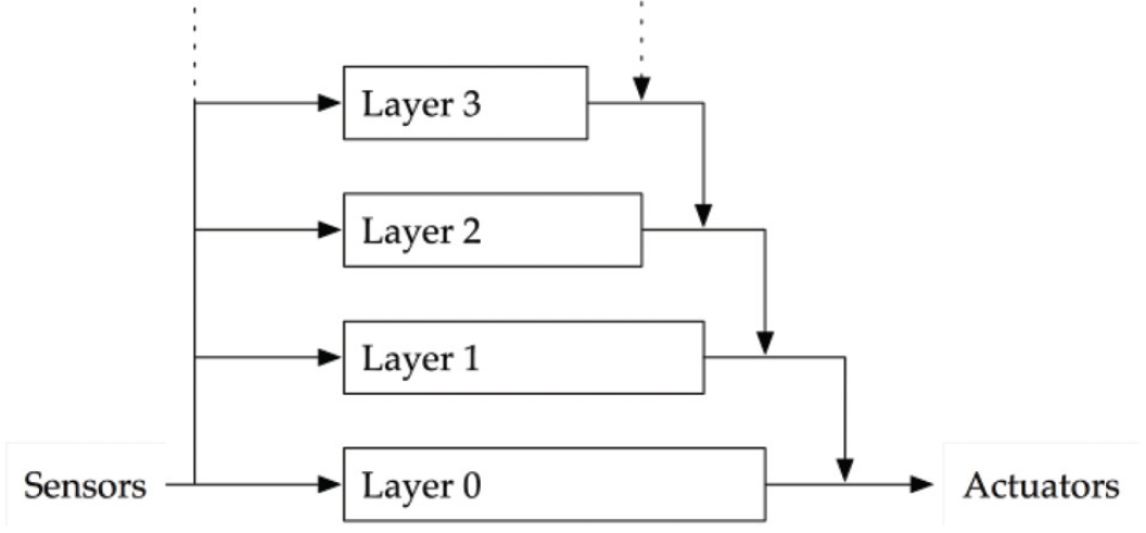
Subsumption architecture control model (diagram adapted from (Brooks, R.A. (1986)))

Each control level consists of a set of behaviours, implemented as a finite state transducer loosely modelled on finite state machines. A behaviour has input and output lines, and variables for data storage. Inputs may come from actuators or other behaviours. Each input line is buffered, making the most recently arrived message on a line always available for inspection. Each module has a special reset input, which switches the FSM to its start state on receipt of a message. States of an FSM are classified as Output, Side Effect, Conditional Dispatch, and Event Dispatch. When in an Output state, the FSM sends a message on an output line and enters a new state. The output message is a function of the inputs and variables. In a Side Effect state, a new state is entered and one of the variables is set to a new value computed as a function of the module's input buffers and variables. In a Conditional Dispatch state, one of two subsequent states is entered, determined by a predicate on the variables and input buffers. In an Event Dispatch state, a sequence of pairs of conditions and states are continuously checked, and when a condition becomes true the corresponding state is entered.

The goal of this architecture is to allow control systems to be made up of independent layers that can run in parallel, and incrementally improved as described above. Each layer, however, can monitor data flowing in lower levels and interfere with the flow of data between behaviours in lower levels by suppressing or inhibiting. This means that although the lower levels are unaware of the existence of the higher layers and can control the robot independently, a higher layer cannot be unaware of the structure of lower levels, unless its inputs and outputs are limited to sensors and actuators. The form of data monitoring, suppression and inhibition in subsumption prevents us from looking at each layer of behaviours as a “black box”, so that although the degree of autonomy of the control system increases with the addition of higher layers, the overall system must still be viewed as a distributed one, made up of many small processing modules. The final block diagram of a control system constructed according to Brooks' architecture must include the internal connections between layers, where one layer monitors or interferes with the internal flow of data in another. Consequently, such a diagram cannot, in fact, have the neatly layered structure suggested in Fig. 2. This can impede the understanding of the control system by other designers, complicating the process of editing and maintaining such systems.

Another characteristic of the subsumption architecture is that suppression is applied only to inputs of a behaviour and inhibition to outputs. Considering that the output of each module is connected to the input of another module, except if directly communicating with the hardware, inhibiting an output is equivalent to suppressing the input of the succeeding module. The same argument holds true for suppression. This means that in practical terms, inhibition and suppression can affect both the input and the output of a module, although in cases where there are both suppressors and inhibitors on a line from an output to an input, their order is significant.

In the architecture proposed by Brooks, although the overall control system is decomposed according to the desired behaviours of the robot, one might argue that each layer must still be decomposed in the traditional manner, and must therefore be complete before the expanded control system can execute.

Published descriptions of the subsumption architecture outline an implemented control system, rather than a general formalism for control systems. For example, the nature of the messages sent from sensors or generated by behaviours is not clearly specified. They are sometimes referred to as “signals”, giving the impression that they are continuous. Elsewhere, there are references to Boolean operations applied to messages, and to variables containing Lisp data structures.

3. Subsumption for Programming Robots by Direct manipulation (SPRD)

In order to design a well defined, visual programming-by-demonstration system, we need a precisely specified control model as a foundation; a “structured programming” equivalent to Brooks' “Fortran”. To that end, in this section we propose a simpler, more streamlined subsumption model, sprd, which is functionally equivalent to Brooks' architecture. In the sprd model, each layer consists of a single behaviour, defined as a Finite State Machine which is likely to be more complex than the transducers comprising the modules in Brooks' model. Layers cannot monitor or interfere with the internal data flow of other layers since there is only one fsm in each layer. However, a higher layer can read output from a lower layer in order to monitor its activity, and may inhibit or suppress the inputs and outputs of the layers below it.

3.1 Behaviours

Behaviours in sprd are implemented as Moore Machines, a well known class of finite state transducers, which we will define here for completeness. A Moore Machine is a 5-tuple (Q, Σ, Δ, δ, Λ, q₀) where Q is a finite set of states, Σ is a finite input alphabet, Δ is a finite output alphabet, q₀ ∈ Q is the initial state, 5 is a function from Q × Σ to Q called the transition function, and X is a function from Q to D called the output function.

A robot behaviour must process values from several different input lines rather than just one, so in order to use Moore Machines to implement behaviours, we must combine several input alphabets. Consequently, to realise a behaviour with n inputs from alphabets A₁, A₂ … A_n, we can define a Moore Machine with input alphabet Σ = A₁ × A₂ × … × A_n. Similarly, if the behaviour has several outputs, the output alphabet of the machine will be the Cartesian product of output alphabets of the behaviour.

A Moore Machine, like an fsm, can be depicted as a state diagram, a directed graph in which input values label edges, and vertices are labelled with both state names and outputs.

Although Moore Machines are adequate for implementing simple behaviours, the implementation they provide may be rather clumsy for more complex ones. Consider, for example, the situation in which an autonomous mobile vehicle detects a pedestrian in its path. The sensor values signifying this event will cause a transition from the current state of the machine to some new state which outputs appropriate commands to actuators, in particular, signals sent to brakes. The degree of braking force to be applied should be a function of the speed and the distance from the pedestrian. The only way to implement such a function in a standard Moore Machine, however, is to provide one target state for each value of braking force, with a corresponding transition from the current state, taken in response to a particular combination of speed and distance values. Essentially, the function is explicitly defined in tabular form. Clearly, this can lead to large and repetitious machines.

This example illustrates a further inadequacy of ordinary Moore Machines, namely, that their input and output alphabets are finite. Although the speed of the robot in our example may be bounded, the set of speed values is not finite. The same can be said for braking force and distance. One could always partition such sets into a large but finite set of subsets, but that would exacerbate the first problem mentioned above. We define Extended Moore Machines to overcome these difficulties. An Extended Moore Machine (emm) is a six-tuple (Q, Σ, Δ, δ, Λ, q₀) where Q, δ, and q₀ are as defined above, Σ and Δ are alphabets which are not necessarily finite, Λ is a function from Q to Γ where Γ is the set of all functions from Σ to Δ, and Λ(q₀) is a constant function.

3.2 The SPRD Control Model

An sprd control system is constructed by starting with a hardware robot with no control program and recursively adding behaviours, each implemented as an emm. A higher level behaviour can monitor the data generated by lower level behaviours by reading their outputs. Outputs from a higher level behaviour can subsume or inhibit the inputs to and outputs from lower level behaviours but not vice versa.

The structure of the sprd model is recursively defined by the diagrams in Fig. 3. In this figure, the grey rectangular icons represent sequences of distinct items: in particular the icons [] represent empty sequences. The arrowed lines represent busses carrying vectors of values. The width of a bus incident on a sequence of items is equal to the size of the sequence, and the i^th wire in the bus carries a value to or from the i^th item in the sequence. Icons representing empty sequences, and busses of zero width are included in Fig. 3 for completeness; however, in later figures illustrating control diagrams for particular control systems, we will omit them. The icons indicate concatenation or splitting of vectors in the direction of the arrow. It is easy to prove by induction on the diagrams in Fig. 3, that in the case of splitting, the points at which a vector is divided are well defined.

Fig. 3.

sprd control system

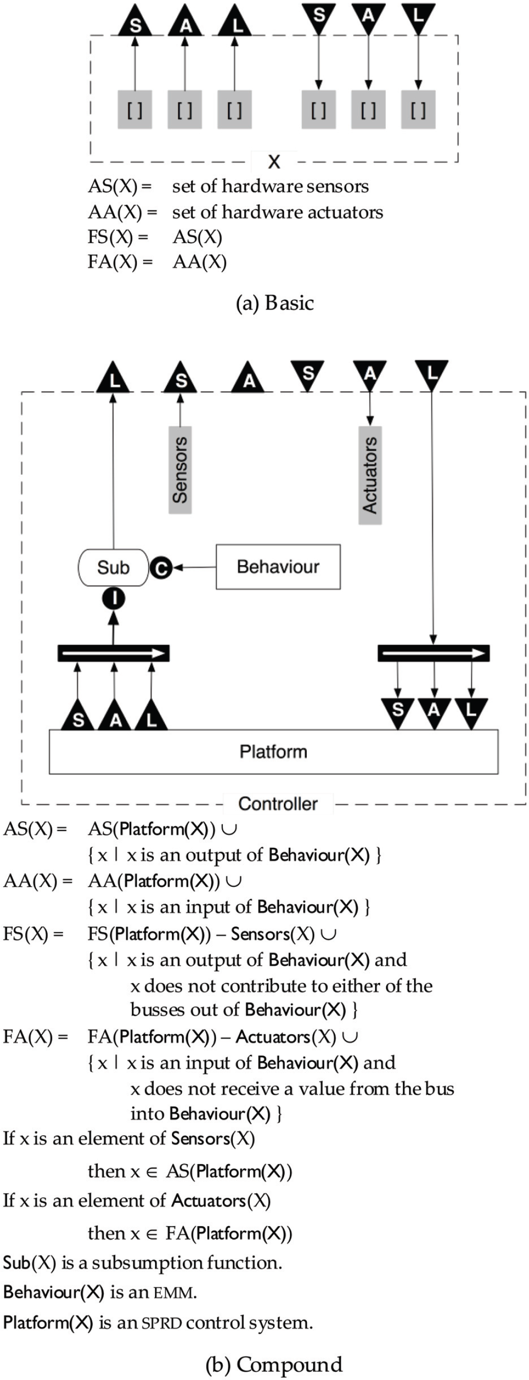
In each of the diagrams in the figure, the labelled arrowheads on the dashed perimeter indicate connections which are not part of the control system being defined, but are necessary for it to function. For example, there is an implicit bus from the to the on the dashed perimeter in each diagram.

The figure defines two kinds of sprd control systems, each consisting of five components: a control diagram, and sets AS, AA, FS and FA of available sensors, available actuators, free sensors and free actuators, respectively. A basic control system performs no computations, and does not interact with the robot's sensors or actuators, but provides the base case for the recursive construction. A compound control system is obtained by combining a behaviour, implemented as an emm, with an existing control system Y in such a way that the behaviour controls, and may override, the actions of Y.

The item Sub in the control diagram of the compound control system in Fig. 3 is a subsumption function. A subsumption function has two vector inputs I and C such that |I| ≥ |C| and produces an output vector of length |I|, such that the i^th component of the output is either the i^th component of the input vector I, or is generated by suppressing the i^th component of I with some component of C, or is generated by inhibiting the i^th component of I with some component of C, and every component of C is used to inhibit or suppress some component of I. Inhibition and suppression are the functions defined in Fig. 1.

If X is a compound sprd control system, the elements of AS(X) and AA(X) which are not hardware sensors or hardware actuators respectively, are called software sensors and software actuators. If X is an sprd control system, we define the level of X to be 0 if X is a basic control system, and 1 plus the level of Platform(X) otherwise.

The intuition behind this definition is as follows. A hardware robot is analogous to a car. It has sensors which, like the gauges on the dashboard of a car, provide information about current conditions, and actuators which, like the controls of a car, can be given values that cause the robot to perform various actions.

A hardware robot, together with an sprd control system, constitutes a robot R, with more capabilities than the bare hardware robot: specifically, it has extra software sensors and software actuators. In order to “run” robot R, we directly connect corresponding output and input pins as described above, whereupon the robot will exhibit the behaviour defined by the control system in the absence of input to the free actuators. We can observe values of sensors, including software sensors, and input values to free actuators, possibly affecting the behaviour.

To extend the capabilities of robot R, we add a processing unit, in the form of an emm, which takes over the function of the human “driver”, reading some of the hardware or software sensors provided by R, and writing values directly to some of the free actuators of R. We can also rewire the external connections between the output and input pins of R, possibly modifying the sensor values that R reads and the actuator values that R writes.

Note that because of the simple form of a level 0 control system, a level 1 control system has the degenerate control diagram shown in Fig. 4, where Sensors and Actuators consist of, respectively, the hardware sensors read by Behaviour, and the hardware actuators controlled by Behaviour. We leave it to the reader to verify that the first level at which the full generality of the model can be realised is 3.

Fig. 4.

Level 1 has a simple form

3.3 Conventions

In order to simplify the emm examples we present later, we introduce some notational conventions.

In a robot control system, an input or output line may or may not carry a signal. The way that a signal or lack of a signal is interpreted will depend on the hardware receiving it. For example, a signal value of 0 input to a motor may have the same effect as no signal at all. In order to support “no signal” values, we define a new no-value symbol η which is included by default in all sets of symbols which are components of input and output alphabets.

The remaining conventions are introduced in order that Moore Machines can be specified in a more compact form, where a single transition may be an abbreviation for a set of transitions.

We define a transition labelled with a set S = {x₁, …, x_n} as an abbreviation for n transitions labelled x₁, …, x_n as shown in Fig. 5.

Fig. 5.

The transition with set label at left is equivalent to the n transitions at right

A Cartesian product X₁ × X₂ × … × X_k is abbreviated as X₁X₂…X_k.

If × is any symbol we will use × to mean {x} when this meaning is clear in context.

The complement of a subset Y is denoted by $\neg γ$ . For example, if the input alphabet of a Moore Machine is , then $\neg {1, 2, η} \neg a \neg ↑$ denotes the set . We extend this notation by applying it to consecutive components of a Cartesian product. For example, $x 1 x 2 \dots x k -_{1} \neg {(x k \dots x_{j})}_{j} + 1 \dots χ_{n}$ denotes the set {x₁} × {x₂} × … × {x_k-1} × (X_kX_k+1…X_j − {x_kx_k+1…x_j}) × {x_j+1} x…x {x_n} where x_i ∈ X_i for k ≤ i ≤ j. The usefulness or applicability of this notation in a particular situation depends on how the components of a Cartesian product are ordered.

If x is an n-tuple then we write x_i to denote the i^th component of x.

In an emm, the output associated with each state is a function of the input value that caused the transition to the state. We use φ to denote the input value that caused this transition. For example, if the output of a state in an emm is the i^th component of the input value, we denote the output by φ_i.

These notations are illustrated in Fig. 6 which depicts EMMs that implement suppression and inhibition. In this figure, the alphabets of the c and i inputs are C and I respectively, and the input alphabet of both machines is CI. The output alphabets of the suppression and inhibition EMMs are $C \cup I$ and I respectively.

Fig. 6.

EMMs implementing suppressor and inhibitor

4. Visual programming for robot control using SPRD

In this section we show how the SPRD model described above can be used as the underlying formalism for SDM, the simulation environment suggested in (Cox, P.T. & Smedley, T.J. (1998)), in which the programmer creates control programs by interacting with a simulation of a robot and its environment. Although the aim of the programming process is to generate an SPRD control system, like other programming-by-demonstration systems, the philosophy of SDM is to focus the programmer's attention on making the simulated robot behave properly, rather than on the underlying abstraction. It is important to note that “demonstrating” an action does not always mean directly illustrating the result of the action. For example, demonstrating how to make an automobile move forward does not entail pushing the car. The demonstration involves giving a value to a control (the accelerator pedal), which will cause the driving wheels to turn, achieving the required result. Similarly, in our proposed PBD environment, the programmer demonstrates behaviour by setting values for the robot's actuators via a panel.

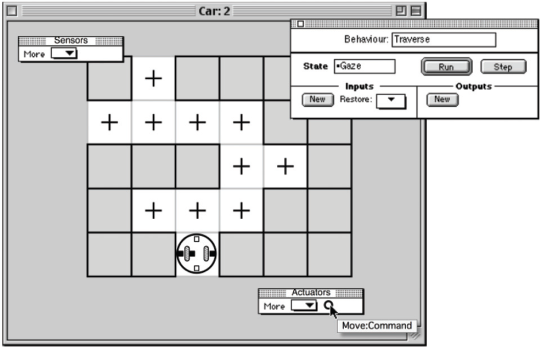
To show how a complete SPRD control system would be created in SDM, we use an example to illustrate the programming steps. The SDM interface we present has not been implemented. Although the interface and example are two-dimensional, the underlying principles are not limited to two dimensions. The example shows how to program a robot car to traverse a maze defined on a rectangular grid. Each grid cell is occupied either by a tile marked with a black cross in the centre, or an obstacle. The car is equipped with two motors and driving wheels, one at each side, and four infrared sensors mounted horizontally at the front, right, left and back, for detecting objects. Another infrared sensor, mounted underneath the robot and slightly to the left, detects the black crosses, and can determine when the car is in the middle of a cell. Because of its left offset, it can also detect when a 90° rotation to the right or left is complete.

Once Car, Tile, and Obstacle are modelled in hdm by a process such as that outlined in (Cox, P.T. & Smedley, T.J. (1998)), the resulting description is loaded into sdm, which displays a workspace window named Car: 0, empty except for an instance of the Car robot, together with a palette of available environment objects. To create an environment for simulation, instances of Tile and Obstacle are created by dragging from the palette into the workspace (Fig. 7), and arranging them into a maze. As the cursor passes over a significant item, such as an actuator or sensor, the name of the item appears, as shown in the figure. After assembling an environment, we close the object palette and begin the programming task. The Car: 0 workspace window is a representation of the basic control system in Fig. 3(a).

Fig. 7.

Assembling the simulation environment

A simple maze-traversal algorithm that a human might use in real mazes, involves walking forward while at all times keeping one hand on a wall. To program the robot with this algorithm, we start by building a useful low-level behaviour which we will call Move, that will form the level 1 behaviour of the control system, and provide a small alphabet of commands that can be used by higher layers to make the robot move forward or backward from one grid position to another, or to rotate 90° clockwise or counterclockwise. Once the Move behaviour has been defined, we will build higher levels to address the maze-traversal task.

4.1. Programming level 1

To define the Move behaviour, we build a level 1 SPRD control system according to the diagram in Fig. 4. First, we select a menu item New Behaviour, which renames the workspace window Car:1, and opens a floating palette as shown in Fig. 8, corresponding to the Behaviour block in Fig. 4. This palette, used to define the inputs, outputs and states of the emm, contains an editable text box where we name the behaviour Move. The name can be edited at any time and has no logical significance, although as we shall see, it is important for building higher level systems that behaviour names are intuitive and distinct from one another.

Fig. 8.

Programming at Level-1

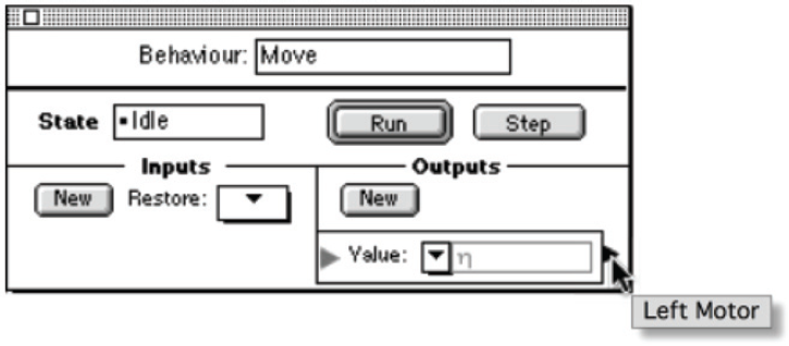
The first step in programming the Move behaviour is to define its initial state, which we name Idle as shown in Fig. 9. The • in the name, indicating that this is the initial state, cannot be deleted. Also, since every behaviour can have only one initial state, only one state can have a name starting with •.

Fig. 9.

Adding an output

The Move behaviour must generate appropriate outputs for both the left and right motors in order to move or rotate the car. To add an output we click the New button for outputs, which adds an output panel, shown in the bottom right corner of the Move palette in Fig. 9. This panel contains an editable text box for the name of the output, initially untitled, a pop-up menu for selecting the type of the output, a function pop-up that specifies how the output value is computed, a popup menu and box for setting the output value, and a connection terminal represented by a small triangle attached to the right of the panel. Since the output has no type to begin with, the function popup is set to Constant, the value box displays η and the function popup, value popup and value box are all disabled. Like the name of the behaviour itself, the name of an output has no logical significance, but can be chosen to improve the readability of the program. We rename the output Left Motor as Fig. 9 shows.

Since this output will generate values for the left motor of the car, we connect it to the left motor by clicking on the terminal of Move:Left Motor and dragging, which creates a “rubber band” connecting the terminal and the cursor. As the cursor passes over any item in the environment to which the terminal can be connected, the item is highlighted and its name appears as shown in Fig. 7. We choose the left motor of the car and release the mouse button, connecting the terminal and left motor as shown in Fig. 10. To relate this result to Fig. 4, we note that the newly created connection establishes that the hardware actuator Car:Left Motor is in the sequence Actuators, and that the output Move:Left Motor is included in the bus from Behaviour to , and from to Actuators .

Fig. 10.

Connecting the Left Motor output to the left motor

As a consequence of creating this connection, the output Move:Left Motor is assigned the type of Car:Left Motor, an iconic type defined in hdm to be the set Motor = {↑, ↓}, the value box remains uneditable and the value and function pop-ups are enabled. We can change the output value by selecting a value from the pop-up; however, since we want the car to remain stationary in the Idle state, we leave η as the output value. In our example, the output values displayed are simply the constant outputs defined for the Idle state. In general, however, the output values are computed by functions, as described in Section 3.1.

Once an output has been defined and connected, we can hide its details in order to reduce the size of the behaviour palette, by clicking the icon beside the name of the output. When an output (or input) is reduced, its name is displayed whenever the cursor passes over its terminal, as shown in Fig. 11. Next we define a second output named Right Motor and connect it to Car:Right Motor in a similar way.

Fig. 11.

Reducing an output

In the Idle state of the Move behaviour, the car should remain still, waiting for a command. To add the command input that the car should observe while in the Idle state, we click the New button for inputs. An input panel is added, similar to an output panel except for the absence of a function popup. We name it Command as shown in Fig. 12. The name of an input, like that of an output, has no logical significance. The Command input will eventually receive its values from higher levels of the control system: during programming of the Move behaviour, however, we will supply its value manually. Before a value other than η can be assigned to this input, a type must be specified. In this case we choose from the type pop-up, invoking a type editor, the details of which are beyond the scope of this paper. With this editor we create an iconic type Command = {↑, ↓, ↷, ↶}. Since we have specified an iconic type, the value pop-up is enabled but the value box remains uneditable.

Fig. 12.

Adding an input

By clicking the Run button on the behaviour palette, we initiate simulation. Since the Idle state is completely “untrained”, it cannot react to the h value for the Command input, so the simulation stops and a window, called the transition dialogue opens as shown in Fig. 13. The popup menu from which to choose the next state is initially set to the current state, Idle in this case. Clearly, this is the correct choice, so we click the Run button which dismisses the dialogue, creates a transition from Idle to Idle under the input value η, and restarts simulation, which continues to run, remaining in the Idle state. Since the outputs for both motors are h, the car remains motionless. If we had clicked the Cancel button, the dialogue would have disappeared, but no transition would have been created and the simulation would not have resumed. The Step button is explained later.

Fig. 13.

After simulation has halted

Now we select ↑ from the value pop-up of the Command input, placing ↑ in the value box. Since the Idle state has not been trained to react to this input, the simulation stops again and the transition dialogue opens. We want to create a new state in which the car will begin to move forward, so we choose New state from the popup menu on the dialogue and click Run. This time when the dialogue disappears, a new state named untitled is created, together with a transition to it from Idle, the simulation follows this transition and stops in state untitled. The state name in the behaviour palette changes to untitled. We rename it Start Forward.

We want the Start Forward state to generate values for the Move:Left Motor and Move:Right Motor outputs that will move the car forward until the sensor Car:Lower IR changes from ■ to □, indicating that the car has moved off the centre of the square. Hence, we set Move:Left Motor and Move:Right Motor to ↑, define a new input, Move:Lower IR and connect it to Car:Lower IR. To relate this to Fig. 4, we note that Car:Lower IR has been added to the sequence Sensors, and included in the bus from Sensors to , and from to Behaviour.

As soon as the connection between the Move:Lower IR input and the Car:Lower IR sensor is established, the value of the sensor, currently ■, appears in the value box of Move:Lower IR. Move:Lower IR also inherits the type IR-Sensor. When in the Start Forward state, the Move behaviour should ignore any further changes in the Move:Command input until it finishes executing ↑. To indicate this, we click the icon in Move:Command, removing it from the behaviour palette. This defines Move:Command as insignificant for the Start Forward state, so that whenever this state is entered during simulation, the Move:Command input panel will disappear. Fig. 14 shows the behaviour palette after the Move:Lower IR input panel has been collapsed. The Restore popup menu in the Inputs section of the palette can be used to return a removed input to the set of active inputs. Note that, even though Move:Lower IR gets its value from Car:Lower IR, its value popup is still active, since in certain situations the programmer needs to override the supplied value, as illustrated later.

Fig. 14.

After defining the Start Forward state

As described above, when restarted, the simulation immediately stops, and we confirm in the transition dialogue that, given the current input ■, the control system should remain in the Start Forward state. When started again, the car moves forward in response to the ↑ outputs to both motors. The underneath sensor immediately moves off the cross on the tile, causing its value to change from □ to ■, and the simulation stops. Since the task of moving the car to the next tile is not complete, we create a new state, name it Forward, and leave both Move:Left Motor and Move:Right Motor set to ↑.

When restarted, the car moves forward until the underneath sensor changes from □ to ■, causing the simulation to stop again. At this point the car has reached the next tile, so processing of the ↑ command is finished. Accordingly, we set the next state to Idle. This time, instead of clicking the Run button on the transition dialogue, we click Step. This creates the transition from Forward to Idle, and advances the simulation by one step to the Idle state. If we had clicked Run rather than Step, the simulation would have resumed after the creation of the new transition, transferred to Idle and immediately begun processing the ↑ command again, driving the car through the obstacle in its path. Next we set value the of the Move:Command input to η and restart the simulation, which continues to run in the Idle state. At this point the workspace appears as in Fig. 15. Note that while the simulation is running, the Run button is renamed Stop, and the Step button is inactive.

Fig. 15.

The state of the simulation after processing the ↑ command.

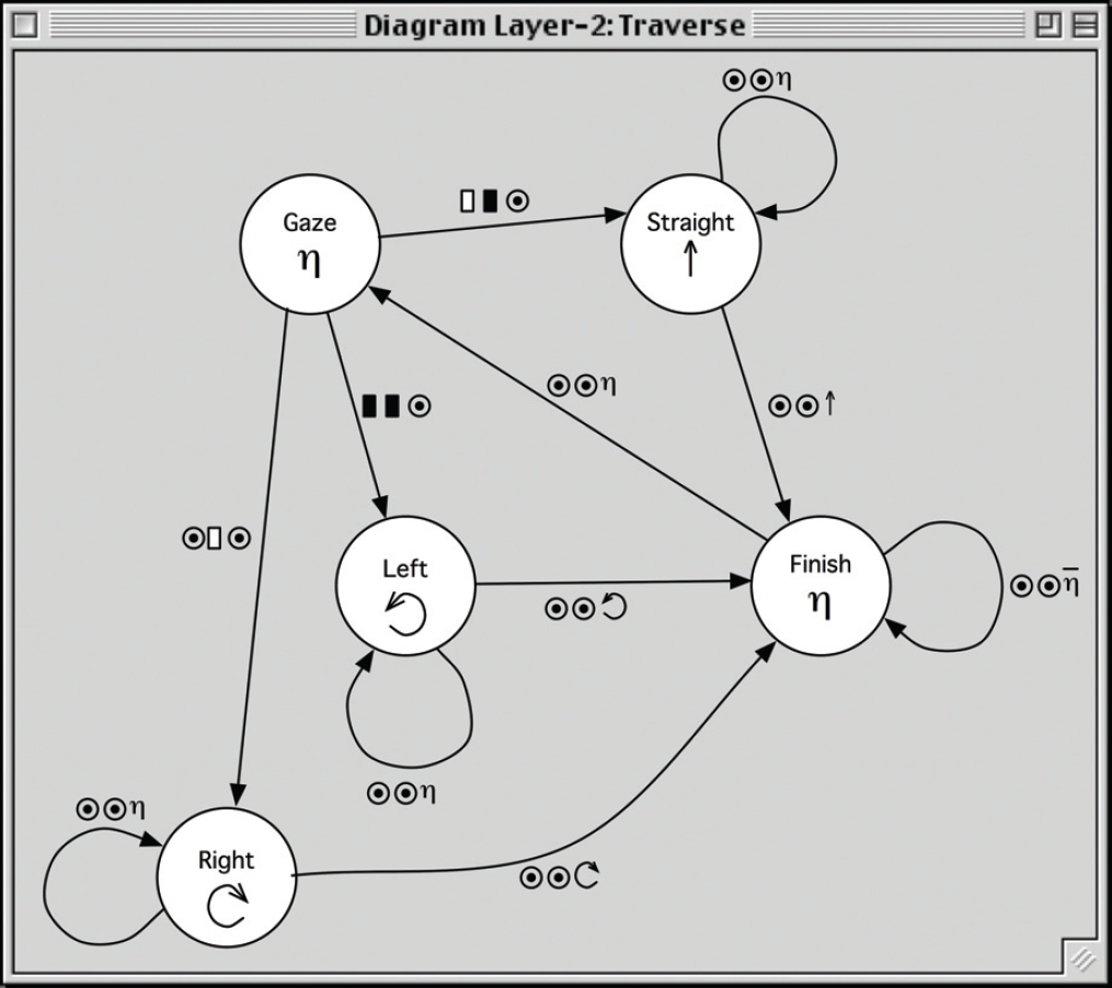
At any time during the process of programming a behaviour, we can select a menu item to open a window displaying the state diagram of the emm generated so far. For example, Fig. 16 shows the state diagram after the Idle, Start Forward, and Forward states have been defined. In this diagram, represents any value from an alphabet. As the cursor passes over an input or output value, the name of the corresponding input or output is displayed, followed by the name of its alphabet, as illustrated in the figure.

Fig. 16.

emm state diagram for Move.

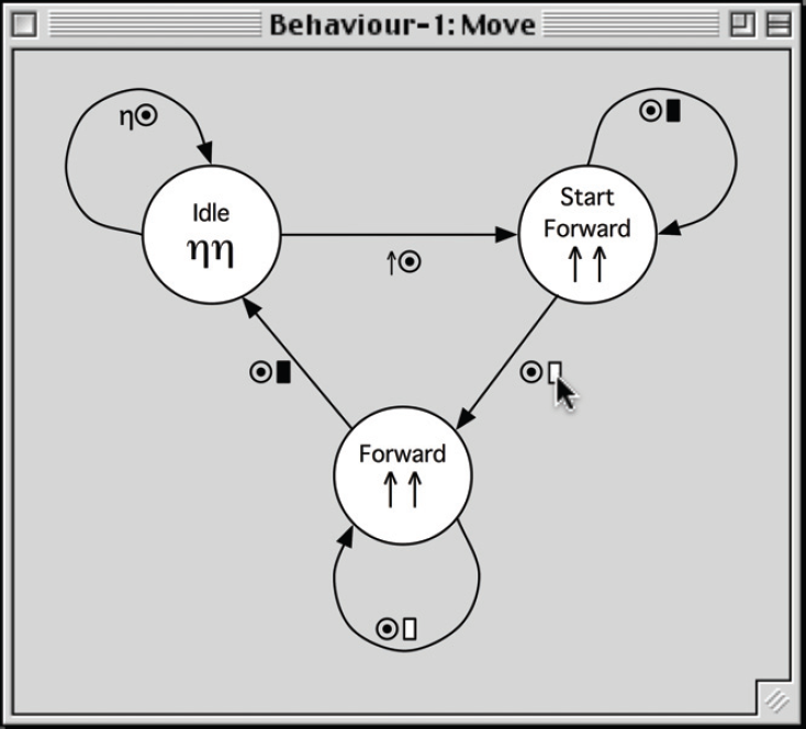
To complete the programming of the Move behaviour, we follow a sequence of steps analogous to the above for each of the remaining command input values ↷, ↶ and ↓, generating states Start Right, Right, Start Left, Left, Start Reverse and Reverse and the connecting transitions. To clarify the function of the Restore popup on the behaviour palette, we note that when the state Start Right is created, the only input on the behaviour palette is Move:Command . We remove the Move:Command input by clicking its icon, and select Lower IR from the Restore menu.

At this point, the simulation runs without stopping, responding appropriately to each of the four possible values for Move:Command . The behaviour we have programmed so far, however, is oblivious to obstacles and sensitive only to the marks in the centre of grid positions. Hence, if allowed to run continuously, it will respond only to changes in Move:Command, perhaps driving the simulated car through obstacles.

To relate the control system developed in this section to the structure defined in Section 3.2, we make the following observations. Note that, as a convenience, we use the name of the behaviour to also identify the control system of which it is a component when the meaning is clear in context.

The control diagram of Move has the form shown in Fig. 4.

Sensors (Move) = [Car:Lower IR]

Actuators (Move) = [Car:Left Motor, Car:Right Motor]

AS(Move) = {Car:Left IR, Car:Right IR, Car:Front IR, Car:Back IR, Car:Lower IR, Move:Left Motor, Move:Right Motor}

AA(Move) = {Car:Left Motor, Car:Right Motor, Move:Command}

FS(Move) = {Car:Left IR, Car:Right IR, Car:Front IR, Car:Back IR}

FA(Move) = {Move:Command}

software sensors of Move = {Move:Left Motor, Move:Right Motor}

software actuators of Move = {Move:Command}

4.2. Programming level 2

Next we build a level 2 control system by adding to level 1 a new behaviour Traverse, which drives the robot through the maze. Instead of driving the motors directly, the Traverse behaviour will send commands to the Move behaviour.

To initiate this construction, we select the menu item New Behaviour. The workspace window is renamed Car:2, the Move behaviour palette and all its connections disappear, a new behaviour palette is opened, representing the new emm, and two palettes named Sensors and Actuators appear. Fig. 17 illustrates the workspace after we have named the new behaviour Traverse, named its initial state Gaze, and moved the robot back to the start of the maze.

Fig. 17.

Creating the Traverse behaviour.

The Sensors and Actuators palettes give access to all software sensors and actuators provided by the platform on which we are building the current behaviour, that is, the Move control system in this example. The Actuators palette initially displays a list of the free software actuators of the platform, represented by small circles. As the cursor passes over each circle, the name of the actuator is displayed together with the name of the associated behaviour, as shown in Fig. 17. The palette also includes a popup menu called More providing access to software actuators of the platform which are not free. Selecting one of these adds a corresponding circle to the palette. The Sensors palette provides access to software sensors in a similar fashion, initially displaying an icon for each free software sensor provided by the platform. The rationale behind this interface is that the software sensors and actuators that are most likely to be of interest are those that have not been used in the platform control system. Note that the hardware sensors and actuators, both free and used, are available directly on the simulated robot.

The function of the Gaze state is to determine what the next action should be, depending on the values of the sensors Car:Front IR and Car:Right IR . As we shall see, these sensors are not monitored in other states of the Traverse behaviour, which are concerned only with generating commands for the Move:Command input, and monitoring outputs of Move to determine when a command has been performed.

For the Gaze state we define an output named Command and, as described above, create a connection from it to the Move:Command software actuator on the Actuators palette. The Traverse:Command output inherits the iconic type Command from the Move:Command actuator. Its Value box and Function popup are initially set to η and Constant, respectively. As explained above, in the Gaze state we simply want to observe the environment, not move the robot, so we leave the value η. Next we add two inputs Front and Right and connect them to the Car:Front IR and Car:Right IR respectively. They inherit the types and values shown in Fig. 18, which illustrates the workspace at this point. When we click the Run button to start simulation, the transition dialogue opens, and we choose to create a new state which we name Straight.

Fig. 18.

Inputs and outputs for the Gaze state.

The Straight state is responsible for initiating forward movement of the car, so we set the Traverse:Command output to ↑. The Straight state must know when the movement has started, but need not be concerned with the values of the two infrared sensors. Accordingly, we remove the Traverse:Front and Traverse:Right inputs, and add a new input called Working that reads the Move:Left Motor . To connect it, we click on the terminal of the input and drag, obtaining a rubber band as described previously. This time, however, we drag the cursor over the More menu of the Sensors palette, the menu expands, and we choose Move: Left Motor as shown in Fig. 19. An icon representing the Move: Left Motor software sensor is added to the Sensors palette with a connection to the Traverse:Working input.

Fig. 19.

Connecting to a software sensor.

When we start the simulation, the transition dialogue immediately appears, and we choose Straight as the next state given input value η. As soon as the Move behaviour begins outputting ↑ to the motors, the left motor in particular, Traverse:Working receives the value ↑ and simulation stops. We create a new state Finish and set its value for the Command output to η. On resuming simulation, we confirm that, given input value ↑, the next state is Finish. The simulation now runs continuously until Move has finished processing the ↑ command. At this point the Traverse:Working input receives the value η, simulation stops and we set the next state to Gaze. The car is now positioned as shown in Fig. 20, so keeping in mind the maze-following algorithm described earlier, we train the robot to turn right. The decision to turn right does not depend on the value of Traverse:Front, but is based solely on the fact that Traverse:Right has the value □. We indicate this by selecting (“don't care”) from the Value popup menu of the Traverse:Front input. If we did not override the sensor value in this way, we would later have to train the robot to turn right for the other applicable sensor combination.

Fig. 20.

After processing the ↑ command.

Once all combinations of input values in the Gaze state have been dealt with, the simulation will proceed without stopping. The resulting emm is shown in Fig. 21. Note that not all possible transitions have been defined: for example there is no transition out of the Straight state for any value of Traverse:Working other than ↑. A diagram may be missing transitions for two reasons. First, it may not be complete: that is, there are input combinations that have not yet been encountered, but could arise. As with any program that does not deal with all possible inputs, this may lead to unpredictable behaviour in future. Second, the diagram may be complete since certain input combinations cannot occur. There are three ways this can arise. An input alphabet may contain values that are never generated: for example, infrared sensors never generate η. Certain input combinations may be precluded by the physical properties of the robot and environment: for example, while the robot is moving forward, the horizontal infrared sensors cannot all become ■. Logical properties of the control program may make certain combinations impossible, as in our example where the value of Traverse:Working in state Straight is determined by the output of Straight.

Fig. 21.

emm state diagram for Traverse.

To relate the control system developed so far to the structure defined in Section 3.2, we note the following.

The control diagram of Traverse is as in Fig. 22.

Sensors (Traverse) = [Car:Front IR, Car:Right IR, Move:Left Motor]

Actuators (Traverse) = [Move:Command]

AS(Traverse) = {Car:Left IR, Car:Right IR, Car: Front IR, Car:Back IR, Car:Lower IR, Move:Left Motor, Move:Right Motor, Traverse:Command}

AA(Traverse) = {Car:Left Motor, Car:Right Motor, Move:Command, Traverse:Front, Traverse:Right, Traverse:Working}

FS(Traverse) = {Car:Left IR, Car:Back IR }

FA(Traverse) = ϕ

software sensors of Traverse = {Move:Left Motor, Move:Right Motor, Traverse:Command}

software actuators of Traverse = {Move:Command, Traverse:Front, Traverse:Right, Traverse:Working}

Fig. 22.

The control diagram of Traverse.

4.3. Programming level 3: subsumption

To conclude our example, we add another level to the control model to illustrate subsumption. This third level implements a controller with which the user can pause and resume the progress of the robot as it traverses the maze. As described above, we create a new behaviour called Controller, rename its initial state Pause, add an input called Control with alphabet Status = {}, set its value to , and add an output called Motors . Next, we connect Controller:Motors to the Car:Left Motor . Since the output Move:Left Motor is already connected to Car:Left Motor, we get an indirect connection from Controller:Motors to Car:Left Motor via a suppressor (see Fig. 6(a)), represented by the arrowhead in Fig. 23. The line from Controller:Motors connects to the c input of the suppressor: the i input is provided by level 2 of the control system, specifically, the output Move:Left Motor . As a consequence of this connection, the output Controller:Motors inherits the type Motor .

Fig. 23.

Creating a subsumption function.

Replacing the level 2 signals to the motors is, however, not what we need to do to make the robot pause: we should simply inhibit the level 2 signals. Accordingly, we double-click the suppressor to transform it into an inhibitor. Controller:Motors reverts to being typeless since it no longer provides a value to the left motor. We set its type to Status, an arbitrary choice since all it needs is a non-empty alphabet. Finally, we connect Controller:Motors to Car:Right Motor via another inhibitor, and set its value to . Fig. 24 illustrates the workspace at this point. Continuing in the manner described in preceding sections, we construct the emm for Controller depicted in Fig. 25. Now when the simulation is running, the robot will stop moving whenever we set Controller:Control to , and resume when we set it to .

Fig. 24.

Inhibiting the output of lower layers.

Fig. 25.

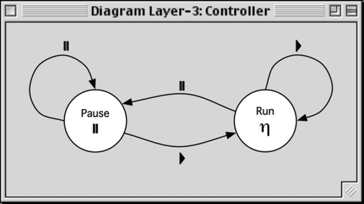
Diagram for Controller.

As in previous sections, we relate the control system developed here to the structure defined in Section 3.2, as follows.

The control diagram of Controller is as in Fig. 26.

Sub(Controller) consists of two inhibitors both with control input Controller:Motors from bus 5, and data inputs Move:Left Motor and Move:Right Motor from bus 3. All other components of busses 1, 2 and 3 pass through to bus 4 unchanged.

Sensors(Controller) = [ ]

Actuators(Controller) = [ ]

AS(Controller) = {Car:Left IR, Car:Right IR, Car:Front IR, Car:Back IR, Car:Lower IR, Move:Left Motor, Move:Right Motor, Traverse: Command, Controller:Motors }

AA(Controller) = {Car:Left Motor, Car:Right Motor, Move:Command, Traverse:Front, Traverse:Right, Traverse:Working, Controller:Control}

FS(Controller) = {Car:Left IR, Car:Back IR}

FA(Controller) = ϕ

software sensors of Traverse = {Move:Left Motor, Move:Right Motor, Traverse:Command, Controller: Motors}

software actuators of Traverse = {Move:Command, Traverse:Front, Traverse:Right, Traverse:Working, Controller:Control}

Fig. 26.

The control diagram of Controller.

4.4. What the example does not show

As discussed in Section 3.1, Extended Moore Machines allow for state outputs to be computed as functions of the input values on incoming transitions in order to deal with large, possibly infinite alphabets. However, to keep the above presentation as straightforward as possible, we have used a simple example in which the input and output alphabets are small. Consequently, this example does not lend itself to a realistic illustration of the use of functions in computing the outputs of states. For the same reason, the example does not demonstrate the construction of transitions corresponding to subsets of input values.

The example also does not illustrate the situation in which the programmer needs access to software sensors and actuators defined at some level below that of the behaviour currently being programmed. Unlike software sensors and actuators defined as outputs and inputs of the current behaviour, these lower-level ones are not directly available with the interface described above. To remedy this deficiency, our proposed environment allows the programmer to create a control panel, a floating palette similar in structure to a behaviour palette. Fig. 27 depicts a control panel imposed on the Traverse SPRD control system. The structure and limitations of our example do not provide a basis for a reasonable use of the control panel, so Fig. 27 simply illustrates the interface, not a meaningful application of it. The control panel has inputs and outputs like a behaviour palette, except that they are referred to as “sensors” and “actuators”, and their names are inherited from the items to which they are connected. A connection from a control panel actuator to an actuator which is not free will introduce a subsumption function, which will have an explicit data input if the pre-existing connection is visible; for example, the suppressor on the connection from the control panel to Traverse:Front in Fig. 27 has a data input from Car:Front IR.

Fig. 27.

Adding a control panel.

In terms of the SPRD model, the control panel is a behaviour in a level above the one currently being simulated, its functionality provided manually rather than by an emm. Clearly, this concept could be extended by providing a library of realistic controls and gauges enabling the construction of realistic control panels similar to the “front panels” of LabVIEW (Johnson, G.W. (2006)).

5. Discussion

In previous sections we noted that Brooks' subsumption model, because of its modularisation of a control system into independent behaviours, provides a foundation for visual language environments for robot control programming, and listed some examples. We also noted characteristics of Brooks' formulation that make it less than ideal for this purpose, motivating the SPRD model presented in Section 3. In particular, although the architecture is layered into increasing levels of competence, higher layered into increasing levels of competence, higher layers can, and may need to, interfere with the flow of data in lower layers, and must therefore be aware of the inner structure of those layers. Hence the levels do not represent levels of abstraction in the software engineering sense, each presenting a well defined interface but hiding its implementation. Furthermore, the behaviours in each layer are interdependent, so cannot be individually tested and debugged. As a result, in order for a user to build a control system in a programming environment based on Brooks' subsumption, he or she would have to be aware of, and be able to directly edit, the underlying structures, as in the vbbl language (Cox, P.T.; Risley, C.C. & Smedley, T.J. (1998)). This need to be aware of underlying structure is at odds with the closeness-of-mapping principle, a mainstay of PBD.

In contrast, the recursive structure of SPRD encourages the programmer to view the programming task as extending an existing robot that provides an interface consisting of sensors and actuators, by adding one new behaviour and defining further, higher-level sensors and actuators. Certain aspects of the SPRD control model still show through in the interface we have proposed. While building a behaviour, the programmer needs to be aware of the concepts of “state” and “transition”: however, these are arguably quite natural concepts in the context of a problem that has a finite state solution. For example, a human walking a maze will be aware of being in the state “walking straight ahead with right hand on wall”, and on encountering a wall, will be aware of the need to start doing something else. Although SPRD reduces the need for the programmer to understand intricate wiring details, he or she must still understand subsumption functions, which are explicitly represented in the interface described above. Because of the simpler structure of the SPRD model, however, the application of subsumption is limited to replacing or turning off a signal from a sensor or a signal to an actuator in the “platform” robot, so is possibly less daunting than subsumption in the Brooks model.

A proof that the recursive structure of SPRD can capture the functionality of the Brooks model is precluded by the fact that Brooks' architecture is not formally defined. Instead we invite the reader to examine the diagram in Fig. 28, depicting one level of a Brooks control system. In this diagram, each node is a behaviour and the edges indicate flows of data between behaviours and between behaviours and the robot hardware.

Fig. 28.

A level 0 control system (adapted from (Brooks R.A. (1986)) Fig. 5).

To create an equivalent control system in SPRD, we would create one of these behaviours first. For example, we may decide to start with forward, which is described as follows: “The Forward module commands the robot to move forward but halts the robot if it receives a message on its halt input line during the motion” (Brooks, R.A. (1986)). In our proposed environment, we would create a level 1 behaviour Forward, similar to Move in Section 4.1, which reads hardware sensors and writes hardware actuators as appropriate to achieve the described behaviour, and implements software actuators Forward:heading and Forward:halt, and a software sensor Forward:encoders . During the development of this behaviour, we would manually supply values for the software sensor. We would add to the functionality of this enhanced robot by building a level 2 system incorporating the behaviour Turn, corresponding to the turn module in the diagram, which would write to the software actuator Forward:heading, read the software sensor Forward:encoders, and implement the software actuator Turn:heading . Clearly, by continuing this process, we can incrementally reproduce the functionality of the diagram in Fig. 28.

The effectiveness of a control model and programming environment such as that we have proposed ultimately needs to be assessed by user testing. We believe, however, that further investigation is necessary before expending resources on implementing a prototype. For example, the behaviours embedded in the recursive structure we have described need not be finite state machines: in fact, other models would be necessary in order to achieve behaviours beyond the simple reactive ones. Preliminary work in this direction focusses on the use of neural networks for implementing behaviours (S.M. & Cox P.T. (2004)). Another possibility to consider is the feasibility of incorporating logic-based control systems to implement deductive behaviours, and the extent to which these parts of a hybrid system might be amenable to visual PBD (Amir, E. & Maynard-Zhang, P. (2004): Lespérance, Y.; Levesque, H.; Lin, F.; Marcu, D.; Reiter, R. & Scherl, R.B. (1994): Poole, D. (1995)).

Footnotes

6.

This work was partially supported by the Natural Sciences and Engineering Research Council of Canada Discovery Grant OGP0000124.

References

Aleotti

Caselli

& Reggiani

(2004) Leveraging on a virtual environment for robot programming by demonstration, Robotics and Autonomous Systems, Vol. 47, Nos. 2–3, (June 2004), pp. 153–161, ISSN 0921-8890.

Ambler

A.L.

Green

Kimura

T.D.

Repenning

& Smedley

T.J.

(1997) Visual Programming Challenge Summary, Proceedings of IEEE Symposium on Visual Languages, Tortora

(Ed.), ISBN 0-8186-8144-6, pp. 11–18, Capri, September 1990, IEEE Computer Society, Los Alamitos, CA.

Amir

& Maynard-Zhang

(2004) Logic-based subsumption architecture, Artificial Intelligence, Vol. 153, No. 1–2, (March 2004), pp. 167–237, ISSN 0004-3702.

Banyasad

(2000) A Visual Programming Environment for Autonomous Robots, MCompSci Thesis, Dalhousie University, Halifax.

Banyasad

Cox

P.T.

& Young

(2000) Constructing Robot Control Programs by Demonstration, Proceedings of Visual End User Workshop, Smedley

(Ed.), Seattle, USA, September 2000, CD only.

Bentivegna

D.C.

Atkeson

C.G.

& Cheng

(2004) Learning tasks from observation and practice, Robotics and Autonomous Systems, Vol. 47, No. 2–3 (June 2004), pp. 163–169, ISSN 0921-8890.

Best

S.M.

& Cox

P.T.

(2004) Programming Autonomous Robots by Demonstration using Artificial Neural Networks, Proceedings of IEEE Symposium on Visual Languages and Human Centric Computing, Bottoni

Hundhausen

Levialdi

Tortora

(Eds.), pp. 157–159, ISBN 0-7803-8696-5, Rome, September 2004, IEEE Computer Society, Los Alamitos CA.

Billard

& Dillmann

(2004) Social mechanisms of robot programming by demonstration, Special Issue, Robotics and Autonomous Systems, Vol. 54, No. 5, (May 2006), pp. 351–352, ISSN 0921-8890

Billard

Epars

Calinon

Schaal

& Cheng

(2004) Discovering optimal imitation strategies, Robotics and Autonomous Systems, Vol. 47, No. 2–3, (June 2004), pp. 69–77, ISSN 0921–8890.

10.

Billard

& Siegwart

(2004) Robot Learning from Demonstration, Special Issue, Robotics and Autonomous Systems, Vol. 47, No. 2–3, (June 2004), pp. 65–67, ISSN 0921-8890.

11.

Brooks

R.A.

(1986) A Robust Layered Control System for a Mobile Robot, IEEE Journal of Robotics and Automation, Vol. 2, No. 1, (March 1986), pp. 14–23, ISSN 0882-4967.

12.

Carrel-Billiard

& Akerley

(1998) Programming with Visual Age for Java, Prentice Hall, ISBN 0-13-911371-1, Englewood Cliffs.

13.

Chella

Dindo

& Infantino

(2006) A cognitive framework for imitation learning, Robotics and Autonomous Systems, Vol. 54, No. 5, (May 2006), pp. 403–408, ISSN 0921-8890.

14.

Cox

P.T.

Risley

C.C.

& Smedley

T.J.

(1998) Toward Concrete Representation in Visual Languages for Robot Control, Journal of Visual Languages and Computing, Vol. 9, No. 2, (April 1998), pp. 211–239, ISSN 1045-926X.

15.

Cox

P.T.

& Smedley

T.J.

(1998) Visual Programming for Robot Control, Proceedings of the 1998 IEEE Symposium on Visual Languages, Smedley

& McIntyre

(Eds.), pp. 217–224, ISBN 0-8186-8712-6, Halifax, September 1998, IEEE Computer Society Press, Los Alamitos, CA.

16.

Cypher

(Ed.) (1993). Watch What I Do: Programming by Demonstration, MIT Press, ISBN 0-262-03213-9, Cambridge MA.

17.

Gindling

Ionnidou

Loh

Lokkebo

& Repenning

(1995) LEGOSheets: A Rule-Based Programming, Simulation and Manipulation Environment for the LEGO Programmable Brick, Proceedings of the IEEE Symposium on Visual Languages, Haarslev

(Ed.), pp. 172–179, ISBN 0-8186-7045-2, Darmstadt, September 1995, IEEE Computer Society, Los Alamitos, CA.

18.

Green

T.R.G.

& Petre

(1996) Usability Analysis of Visual Programming Environments: A ‘Cognitive Dimensions’ Framework. Journal of Visual Languages and Computing, Vol. 7, No. 2, (June 1996), pp. 131–174, ISSN 1045-926X.

19.

Jackson

& Eddy

(1999) Design and Implementation Methodology for Autonomous Robot Control Systems, International Submarine Engineering Ltd., Available from http://www.ise.bc.ca/robotics-paper.html, Accessed: 2007-09-11.

20.

Johnson

G.W.

(2006) LabVIEW Graphical Programming, 4th edn., McGraw-Hill, ISBN 0-07-145146-3, New York.

21.

Kahn

(1996). Seeing systolic computations in a video game world, Proceedings of IEEE Symposium on Visual Languages, Burnett

& Citrin

(Eds.), pp. 95–101, ISBN 0-8186-7510-1, September 1996, Boulder, CO, IEEE Computer Society, Los Alamitos, CA.

22.

Kahn

(2000) Programming by example: generalizing by removing detail. Communications of the ACM, Vol. 43, No. 3, (March 2000), pp. 104–106, ISSN 0001-0782.

23.

Lau

(2001) Programming by Demonstration: a Machine Learning Approach, PhD thesis, University of Washington, Seattle WA.

24.

Lespérance

Levesque

Lin

Marcu

Reiter

& Scherl

R.B.

(1994) A logical approach to high-level robot programming - a progress report, Working notes of AAAI Fall Symposium on Control of the Physical World by Intelligent Systems, Kiupers

(Ed.), pp. 79–85, ISBN 978-0-929280-77-6, November 1994, New Orleans, LA, AAAI Press, Meno Park, CA.

25.

Lieberman

(1993) Tinker: a programming by demonstration system for beginning programmers, Iin: Watch what I do: programming by demonstration, Cypher

(Ed.), pp. 49–64, MIT Press, ISBN 0-262-03213-9, Cambridge MA.

26.

Lieberman

Nardi

& Wright

(1999) Training Agents to Recognize Text by Example, Proceedings of the Third International Conference on Autonomous Agents, Etzioni

Müller

J.P.

& Bradshaw

J.M.

(Eds.), pp. 116–122, ISBN:1-58113-066-X, May 1999, Seattle WA, ACM Press, New York NY.

27.

Michail

(1998) Imitation: An Alternative to generalization in Programming by Demonstration Systems, Technical Report UW-CSE-98-08-06, University of Washington, Seattle WA.

28.

Myers

& Buxton

(1986) Creating Highly Interactive and Graphical User Interfaces by Demonstration, Proceedings of 13th International Conference on Computer Graphics and Interactive Techniques, Evans

D.C.

& Athay

R.J.

(Eds.), pp. 249–258, ISBN 0-89791-196-2, Dallas, TX, ACM Press, New York NY.

29.

Myers

& McDaniel

(2001) Demonstrational Interfaces: Sometimes You Need a Little Intelligence; Sometimes You Need a Lot, In: Your Wish is My Command, Lieberman

, (Ed.), pp. 45–60, Morgan Kaufmann, ISBN 1-55860-688-2, San Francisco CA.

30.

NASA Jet Propulsion Laboratory (2007) Spacecraft: Surface Operations: Rover, available http://marsrovers.jpl.nasa.gov/mission/spacecraft_surface_rover.html, Accessed 2007-09-09.

31.

Pfeiffer

J.J.

(1999) A Language for Geometric Reasoning in Mobile Robots, Proceedings of IEEE Symposium on Visual Languages, Hirakawa

& Mussio

(Eds.), pp. 164–169, ISBN 0-7695-0216-4, Tokyo, September 1999, IEEE Computer Society, Los Alamitos CA.

32.

Pfeiffer

J.J.

(1997) A Rule-Based Language for Small Mobile Robots, Proceedings of IEEE Symposium on Visual Languages, Tortora

(Ed.), ISBN 0-8186-8144-6, pp. 162–163, Capri, September 1990, IEEE Computer Society, Los Alamitos, CA.

33.

Poole

(1995) Logic Programming for Robot Control, Proceedings of 14th International Conference on Artificial Intelligence, Mellish

C.S.

(Ed.), ISBN 1558603638, pp. 150–157, Montreal, August 1995, Morgan Kaufmann, San Mateo, CA.

34.

Repenning

(1995) Bending the Rules: Steps Toward Semantically Enriched Graphical Rewrite Rules, Proceedings of the IEEE Symposium on Visual Languages, Haarslev

(Ed.), pp. 226–234, ISBN 0-8186-7045-2, Darmstadt, September 1995, IEEE Computer Society, Los Alamitos, CA.

35.

Simmons

Goodwin

Haigh

K.Z.

Koenig

& O'Sullivan

(1997) A Modular Architecture for Office Delivery Robots, Proceedings of Autonomous Agents '97, Johnson

W.L.

(Ed.), pp. 245–252, ISBN 0897918770, Marina del Rey CA, February 1997, ACM Press, New York NY.

36.

Smith

D.C.

Cypher

& Spohrer

(1994) KidSim: Programming Agents Without a Programming Language. Communications of the ACM, Vol. 37, No. 3 (July 1994), pp. 54–68, ISSN 0001-0782.

37.

St. Amant

Lieberman

Potter

& Zettlemoyer

(2000) Visual Generalization in Programming by Example, Communications of the ACM, Vol. 43, No. 3, (March 2000), pp. 107–114, ISSN 0001-0782.

38.

Steinman

S.B.

& Carver

K.G.

(1995) Visual Programming with Prograph CPX, Manning Publications, ISBN 1884777058, Greenwich CT.

39.

Stone

H.W.

(1996) Mars Pathfinder Microrover: A Small, Low-Cost, Low-Power Spacecraft, Proceedings of the AIAA Forum on Advanced Developments in Space Robotics, Madison, WI, August 1996.

40.

Whitley

K.N.

& Blackwell

A.F.

(2001) Visual Programming in the Wild: A Survey of LabVIEW Programmers. Journal of Visual Languages and Computing, Vol. 12, No. 4, (August 2001), pp. 435–472, ISSN 1045-926X.

41.

Wolber

(1997) Pavlov: An Interface Builder for Designing Animated Interfaces. ACM Transactions on Computer-Human. Interaction, Vol. 4, No. 4 (December 1997), pp. 347–386., ISSN 1073-0516.

42.

Zheng

(1992) Layered Control of a Practical AUV, Proceedings of IEEE Symposium on Autonomous Underwater Vehicle Technology, pp. 142–147, ISBN 0780307054, Washington DC, June 1992, IEEE Press, Piscataway, NJ.

Visual Programming of Subsumption-Based Reactive Behaviour

Abstract

Keywords

1. Introduction

2. Robots and control models

2.1. Brooks' Subsumption Architecture

3.1 Behaviours

3.2 The SPRD Control Model

Footnotes

6.

References