Soil Parameter Identification and Driving Force Prediction for Wheel-Terrain Interaction

Abstract

This paper considers wheeled vehicles traversing unknown terrain, and proposes an approach for identifying the unknown soil parameters required for vehicle driving force prediction (drawbar pull prediction). The predicted drawbar pull can potentially be employed for traversability prediction, traction control, and trajectory following which, in turn, improve overall performance of off-road wheeled vehicles. The proposed algorithm uses an approximated form of the wheel-terrain interaction model and the Generalized Newton Raphson method to identify terrain parameters in real-time. With few measurements of wheel slip, i, vehicle sinkage, z, and drawbar pull, DP, samples, the algorithm is capable of identifying all the soil parameters required to predict vehicle driving forces over an entire range of wheel slip. The algorithm is validated with experimental data from a wheel-terrain interaction test rig. The identified soil parameters are used to predict the drawbar pull with good accuracy. The technique presented in this paper can be applied to any vehicle with rigid wheels or deformable wheels with relatively high inflation pressure, to predict driving forces in unknown environments.

1. Introduction

Wheeled vehicles traversing rough unknown terrain has many potential applications, including defence, agriculture, mining, and space exploration. Most wheeled vehicles still operate under driver supervision while carrying out tasks. Knowledge of the terrain characteristics helps the driver to have a better control of the vehicle.

From wheel-terrain interaction dynamics, it is seen that soil parameters play a vital role in determining vehicle drawbar pull which can, in turn, be utilized for developing traversability prediction criteria and traction control algorithms.

Research on wheel-terrain and track-terrain interactions has progressed since Bekker started pioneering this area (Bekker G., 1956), (Bekker G., 1969). Iagnemma and Dubowsky focused on the characteristics of a rigid wheel in deformable terrain for planetary rover applications (Iagnemma K. & Dubowsky S., 2002), (Iagnemma & et.al., 2004). In (Hutangkabodee S. & et.al., 2007), soil parameter identification for a tracked vehicle traversing unknown terrain is presented. Soil parameter estimation for a wheeled vehicle traversing deformable terrain was first carried out by Iagnemma and Dubowsky (Iagnemma K. & Dubowsky S., 2002). A Linear Least Square estimator was employed as an on-line identification method to identify two key soil parameters, cohesion (c) and internal friction angle (φ), using on-board rover sensors.

In this paper, for the first time, a method for identifying all five soil parameters is proposed for wheel-terrain interactions. The method is an extension from (Hutangkabodee S. & et.al, 2006) where three soil parameters were identified.

The Composite Simpson's Rule (CSR) is used to approximate the integrals of the original wheel-terrain interaction model, as they cannot be integrated analytically. By doing this, the speed of the algorithm increases by a factor of 9. The Generalized Newton Raphson (GNR) method is applied to the modified nonlinear wheel-terrain interaction model for soil parameter identification. This method has been shown to identify unknown parameters with high accuracy and rapid convergence (Zweiri Y.H. & et.al., 2004).

The experimental data from the wheel-terrain interaction test rig (Section 4) and the actual parameters of the experimental soils (obtained by methods described in Section 5) are used to validate the proposed algorithm. The test results show good identification accuracy for all the soil parameters except the pressure-sinkage parameters (S and n) for Garside 60 soil. The reason for the high errors is described in Section 6. The identified soil parameters are used to predict DP over the entire wheel slip range showing good agreement with the measured values. The predicted DP can be used for vehicle performance optimization, traversability prediction, traction control, and trajectory planning.

2. Governing Model

The analytical model of a wheeled vehicle interacting with an unknown deformable terrain is presented in this section, Fig. 1. In this figure, the wheel of a wheeled vehicle is considered rigid. For constant vehicle forward velocity, considering the force balance in the horizontal direction gives (Iagnemma K. & Dubowsky S., 2002):

$$DP=rb\left({\displaystyle \underset{{\theta }_2}{\overset{{\theta }_1}{\int }}\tau (\theta )\cos \theta .d\theta -}{\displaystyle \underset{{\theta }_2}{\overset{{\theta }_1}{\int }}\sigma (\theta )\sin \theta .d\theta }\right),$$

(1)

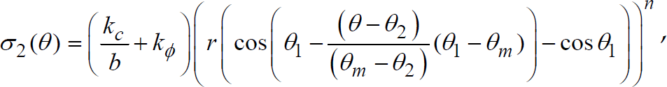
where, DP is the drawbar pull applied to the wheel from the suspension system, θ is the wheel-terrain contact angle measured from vertical axis, θ₁ is the angle at which the wheel first makes contact with the terrain, θ₂ is the angle at which the wheel loses the contact from the terrain, σ is the radial stress normal to the wheel-terrain contact, τ is the shear stress tangent to the wheel-terrain contact, r is the wheel radius, b is the wheel tread, z is the sinkage of the wheel under the terrain surface, θ _m is the angle at which the maximum radial stress occurs, σ₁ is the radial stress profile between θ₁ and θ _m , and σ₂ is the radial stress profile between θ _m and θ₂.

Fig. 1.

Free body diagram of a rigid wheel on deformable terrain (Iagnemma K. & et.al., 2004)

θ₂ is assumed to be zero and the location of the point of maximum radial stress, θ _m , is assumed to be in the middle between θ₁ and θ₂ (Iagnemma K. & et.al, 2004); therefore, θ _m is equal to θ₁/2. The model for soil parameter identification, (1), then becomes (Iagnemma K. & et.al, 2004):

$$DP=rb\left({\displaystyle \underset{0}{\overset{{\theta }_m}{\int }}{\tau }_2(\theta )\cos \theta .d\theta +}{\displaystyle \underset{{\theta }_m}{\overset{{\theta }_1}{\int }}{\tau }_1(\theta )\cos \theta .d\theta -}{\displaystyle \underset{0}{\overset{{\theta }_m}{\int }}{\sigma }_2(\theta )\sin \theta .d\theta }-{\displaystyle \underset{{\theta }_m}{\overset{{\theta }_1}{\int }}{\sigma }_1(\theta )\sin \theta .d\theta }\right),$$

(2)

where,

$${\sigma }_1(\theta )=\left(\frac{k_c}{b}+k_{\varphi }\right){\left(r\left(\cos \theta -\cos {\theta }_1\right)\right)}^n,$$

(3)

$${\sigma }_2(\theta )=\left(\frac{k_c}{b}+k_{\varphi }\right){\left(r\left(\cos \left({\theta }_1-\frac{(\theta -{\theta }_2)}{{\theta }_m-{\theta }_2}({\theta }_1-{\theta }_m)\right)-\cos {\theta }_1\right)\right)}^n,$$

(4)

τ₁(θ) and τ₂(θ) are derived from

$$\tau (\theta )=(c+\sigma (\theta )\tan \varphi )\left(1{-}^{-\frac{r}{K}[({\theta }_1-\theta )-(1-i)(\sin {\theta }_1-\sin \theta )]}\right)$$

(5)

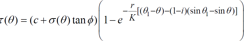
at σ(θ) = σ₁(θ) and σ₂(θ) respectively.

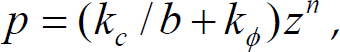
In (3), (4), and (5), k _c , k_φ, and n are the pressure-sinkage coefficients of the soil. These parameters have been derived for terramechanic applications and they characterize normal pressure from a vehicle with sinkage in the soil. c and φ are the soil cohesion, and internal friction angle, respectively. These two parameters characterize the strength of a soil when exposed to axial and shearing loads. K is the shear deformation modulus of the soil and characterizes displacement behavior of the soil under shear forces from a driven wheel.

All four integral terms of the DP model, (2), cannot be integrated analytically. The Composite Simpson's Rule (CSR) is applied to find an approximation to these integrals in order to facilitate the implementation of the identification algorithm and increase the identification speed.

For the integral $\underset{a}{\overset{b}{\int }}f(x)dx$ , suppose that the interval [a, b] is subdivided into 2m subintervals of equal width $h=\frac{b-a}{2m}$ , by using the equally spaced sample points x _k = x₀ + kh for k = 0, 1, 2, …, 2m. The Composite Simpson's Rule for 2m subintervals is given by:

$$E(f,h)=\frac{h}{3}\left(f(a)+f(b)\right)+\frac{2h}{3}{\displaystyle \sum _{k=1}^{m-1}f\left(x_{2k}\right)+\frac{4h}{3}}{\displaystyle \sum _{k=1}^{m}f\left(x_{2k-1}\right).}$$

(6)

The drawbar pull (DP) based on the Composite Simpson's Rule (CSR) approximation and the DP based on numerical integration are shown in Fig. 2. It is observed from this figure that the CSR gives a very accurate approximation of the DP model with an rms error = 0.22 %. In deriving the DP curves in Fig. 2, it is found that while the numerical integration takes 0.045 s, the CSR approximated model takes only 0.005 s. Therefore, this new approximate DP model is more suitable for soil parameter identification in real-time.

Fig. 2.

Comparison of the DP using the CSR approximation and numerical integration

The pressure-sinkage coefficient, k _c /b + k_φ, is a constant, for constant b values. Since in current applications the wheel tread b of a vehicle is constant, a lumped pressure-sinkage coefficient, S = k _c /b + k_φ, is used in (2) and will be treated as a single soil parameter.

3. Soil Parameter Identification Based on the Generalized Newton Raphson (GNR) Method

The proposed soil parameter identification algorithm for wheeled vehicles traversing unknown terrain is based on the Generalized Newton Raphson (GNR) method. This method is well suited for real-time parameter identification since it has been shown to identify unknown parameters with high accuracy and rapid convergence (Zweiri Y.H. & et.al., 2004).

The concept of the GNR method is based on the Newton Raphson (NR) method. The NR method works by iteratively modifying an initial estimate and, after a number of iterations, arrives at a converged solution. Commonly, the iterative process is halted when the error between the identified value and the current value falls below a predefined threshold. The main difference between the GNR and the NR methods is that the NR method employs the same number of equations as the number of unknowns whereas the GNR method uses more equations than the number of unknowns.

The GNR method has the same advantages as those of the NR method, namely its ability to identify unknown individual parameters, its robustness to noise and its fast speed of convergence. In addition, the robustness of the GNR method is even better than that of the NR method (Zweiri Y.H. & et.al., 2004) because it considers more measured data points than the number of unknowns. The GNR method also allows us to use all the measured data available (instead of having to pick 5 data points from maybe 10 available data points as in the NR method case), and thus helps further improve the identification accuracy. However, it is noted that if the initial estimate is selected at a point where the derivative of the function is relatively small, the convergence speed may be slow (Faires J.D. & Burden R, 2003).

The GNR method is implemented to identify the soil parameters for vehicle wheel-terrain interaction dynamics, Fig. 3. Here, vector p comprises five parameters, the cohesion (c), the internal friction angle (φ, the shear deformation modulus (K), the lumped pressure-sinkage coefficient (S), and the pressure-sinkage exponential (n). The vector x consists of three measured signals, drawbar pull (DP), sinkage (z), and wheel slip (i).

Fig. 3.

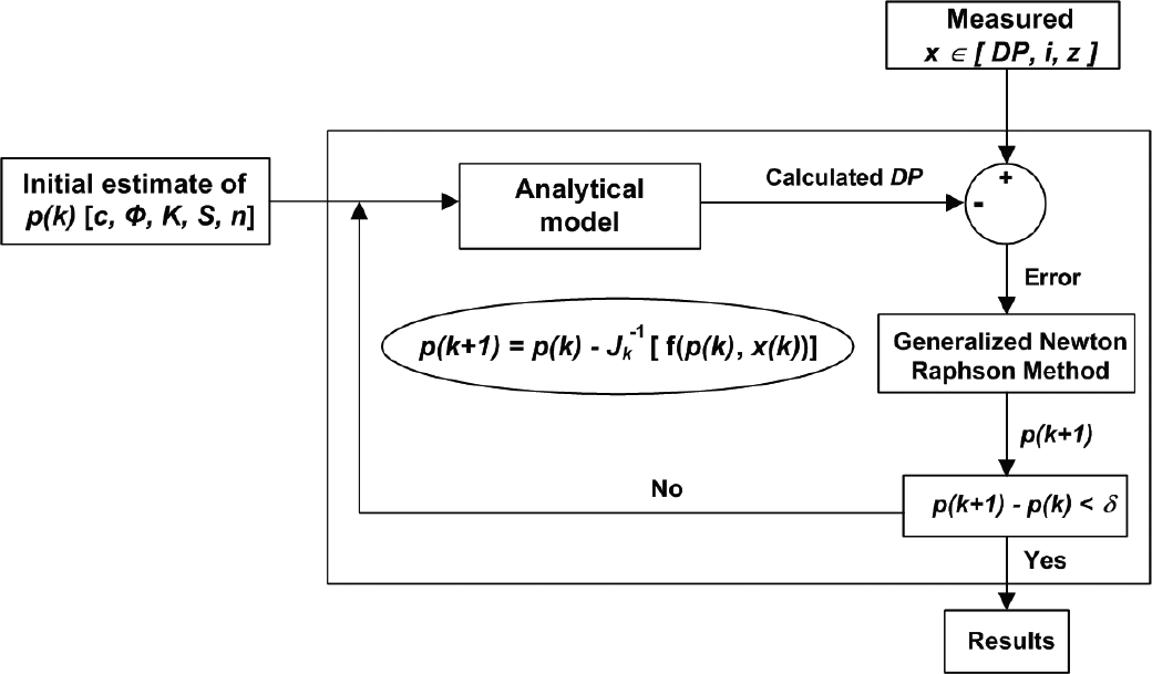
Diagram showing implementation of the GNR method for soil parameter identification

The Composite Simpson's Rule modified wheel-terrain interaction model of (2), and the measurement vector x are used to identify the unknown soil parameters. To find p, q independent equations are required (q ≥ 5). These equations are generated by evaluating the function f at q different time samples (t₁, t₂, …, t _q ). This results in q nonlinear equations expressed in matrix form as:

$$\left[\begin{array}{c}{f}_1(c,\varphi ,K,S,n,D{P}_1,z_1,i_1)\\ f_2(c,\varphi ,K,S,n,D{P}_2,z_2,i_2)\\ ⋮\\ f_q(c,\varphi ,K,S,n,D{P}_q,z_q,i_q)\end{array}\right]=0,$$

(7)

where, p = [c, φ, K, S, n] ^T , and x = [DP, z, i] ^T .

Let $p_0={[c,\varphi ,K,S,n]}_0^T$ be an initial estimate of the unknown parameters. Applying the GNR method to (7) yields:

$$\left[\begin{array}{c}c\\ \varphi \\ K\\ S\\ n\end{array}\right]={\left[\begin{array}{c}c\\ \varphi \\ K\\ S\\ n\end{array}\right]}_0-J_k^{-1}\left[\begin{array}{c}{f}_1(c,\varphi ,K,S,n,D{P}_1,z_1,i_1)\\ f_2(c,\varphi ,K,S,n,D{P}_2,z_2,i_2)\\ ⋮\\ f_q(c,\varphi ,K,S,n,D{P}_q,z_q,i_q)\end{array}\right],$$

(8)

where, $J_k^{-1}$ is the pseudo inverse of J _k since J _k is not a square matrix.

$$J_k=\left[\begin{array}{ccccc}\frac{\partial f_1}{\partial c}& \frac{\partial f_1}{\partial \varphi }& \frac{\partial f_1}{\partial K}& \frac{\partial f_1}{\partial S}& \frac{\partial f_1}{\partial n}\\ \frac{\partial f_2}{\partial c}& \frac{\partial f_2}{\partial \varphi }& \frac{\partial f_2}{\partial K}& \frac{\partial f_2}{\partial S}& \frac{\partial f_2}{\partial n}\\ ⋮& ⋮& ⋮& ⋮& ⋮\\ \frac{\partial f_q}{\partial c}& \frac{\partial f_q}{\partial \varphi }& \frac{\partial f_q}{\partial K}& \frac{\partial f_q}{\partial S}& \frac{\partial f_q}{\partial n}\end{array}\right].$$

4. Test Rig and Experimentation Procedure

The wheel-terrain interaction test rig used in this study is shown in Figs. 4 and 5.

Fig. 4.

Wheel-terrain interaction test rig (1): where, A is the wheel assembly, B is the motor-gearbox-encoder assembly for driving carriage, C is the chain, D are the shafts connected from the top of wheel assembly, E is the carriage, F is the potentiometer, G is the test rig frame, and H is the experimental soil

Fig. 5.

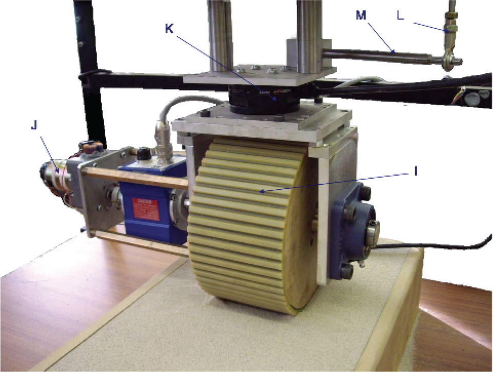
Wheel-terrain interaction test rig (2): where, I is the rigid wheel, J is the wheel motor-gearbox-encoder, K is the Gamma 6-Axis force/torque transducer, L is the moving part of the potentiometer for measuring distance (called “wiper”), and M is the connecting rod for potentiometer's wiper and wheel assembly.

This test rig is developed to test the algorithm proposed in Section 3 in a controlled environment allowing us to acquire all needed parameters in a simple and straightforward manner, and to test the feasibility and effectiveness of the soil parameter identification algorithm. In particular, it is difficult to measure slip parameters on a real vehicle manoeuvring through terrain. Based on current developments in slip estimation (Le A.T., 1999), (Song Z. & et.al., 2005), (Ohno K. & et.al., 2003), (Barshan B. & Durrant-Whyte H.F., 1995), (Chhaniyara S. & et.al., 2006), we assume slip to be measurable on-line enabling the implementation of the proposed soil parameter identification process. With this test rig, the wheel slip, i, the wheel sinkage, z, and the drawbar pull, DP, can be measured very accurately. This allows the soil parameter identification algorithm to be validated in an effective way.

In practice, the signals needed for soil parameter identification in real wheeled vehicles can be acquired as follows. To measure the drawbar pull (DP) of the vehicle, a single-axis force sensor can be installed between the wheel and the vehicle suspension to measure the resultant force in the vehicle heading direction. The vehicle sinkage, z, can be acquired by measuring the gap between axle of driven wheel and ground. Ultrasonic sensors (facing downwards) attached to the vehicle suspension system can be employed for this purpose.

Slip is estimated by employing a sliding-mode observer whose inputs are wheel angular speeds and vehicle heading speed (Song Z. & et.al., 2005). The wheel angular speeds can be measured by attaching either shaft encoders or tachometers onto vehicle wheels' shafts. The vehicle heading speed can be obtained using several techniques such as Global Positioning System (GPS), Inertial Navigation System (INS) (Barshan B. & Durrant-Whyte H.F., 1995), and Optical Flow (Chhaniyara S. & et.al., 2006).

The test rig consists of a driven wheel mounted on a horizontal driven carriage. The wheel is not vertically constrained and can move freely in the vertical direction. The wheel assembly is connected to the carriage assembly using 2 shafts. During experimentation, two motors - one driving the wheel and another driving the carriage - are operated simultaneously at different speeds to generate wheel slip. By varying the differential speeds between the wheel and the carriage motors, various controlled wheel slips can be generated. The test rig is equipped with various sensors to acquire all the measured signals needed for soil parameter identification. Two optical encoders are used to measure the angular speeds of the wheel motor and chain motor. The wheel slip can then be calculated using (9).

$$i=1-r_c{\omega }_c/r_w{\omega }_w,$$

(9)

where, i is the wheel slip, r _w is the wheel radius, r _c is the chain sprocket gear radius, ω _w is the wheel angular velocity, ω _c is the chain sprocket gear angular velocity.

A Gamma ATI 6-Axis force/torque (F/T) transducer mounted between the wheel assembly and the horizontal carriage is used to acquire the drawbar pull, DP. The sinkage (z) of the wheel is measured by a potentiometer. The wheel used in the experiment is 0.1 m in width and 0.2 m in diameter. The test rig is fixed to a 1 m × 1 m × 0.5 m frame. The experimental soil is contained in a 0.3 m × 0.85 m × 0.1 m soil box. Experiments were performed on two types of soils - Garside 60 soil, and Garside iron sand. These soils were purchased from the Garside Sands Company, UK.

5. Acquisition of Soil Parameters for Validation Purpose

5.1. Parameters c and φ

To obtain the cohesion, c, and internal friction angle, φ, of the experimental soils, the Direct Shear Test is conducted (Terzaghi K., 1948). The test is performed on three specimens from a relatively undisturbed soil sample. A specimen is placed in a shear box which possesses two stacked rings to hold the sample. A normal load is applied vertically to the specimen (creating a certain normal stress to the specimen). The upper ring is pulled laterally until the sample fails and the maximum shear stress is then recorded.

Another two different normal loads are applied to another two specimens for the same soil type. The specimens are again sheared until failed and the corresponding maximum shear stresses are stored. The results for these three specimens (normal stress-shear stress values) are plotted on a graph with shear stress as the y-axis and normal stress as the x-axis, Fig. 6. The y-intercept of the experimental curve represents c, and the slope of the curve is φ of the tested soil.

Fig. 6.

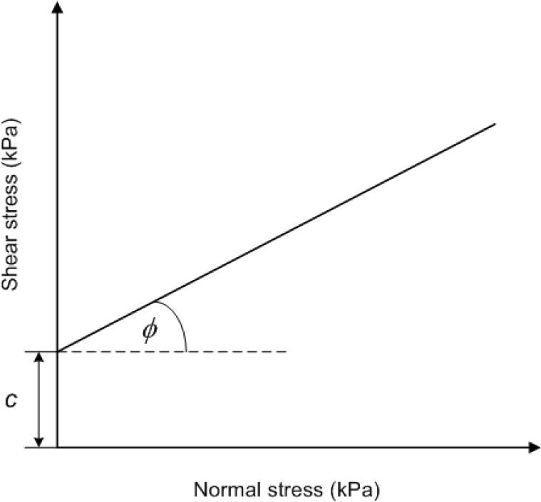
Shear stress vs. normal stress plot and definitions of c and φ

5.2. Parameters k_c, k_φ, and n

The pressure-sinkage parameters k _c , k_φ, and n of the experimental soils are described in the following formula:

$$p=(k_c/b+k_{\varphi })z^n,$$

(9)

where, p is the pressure exerted to the soil, b is the diameter of a circular disc used as the contact area to the soil (or the width of a rectangular plate), z is the corresponding sinkage of the disc into the soil.

Equation (9) characterizes the sinking behavior of a soil when vertically pressed with a circular disc or a rectangular plate. To obtain all three parameters (k _c , k_φ, and n), two discs/plates with different diameter/width are required. Equations (10) and (11) show two sets of equations employed for this purpose (with logarithmic operation applied on both sides of the equation).

$$\log (p)=\log (k_c/b_1+k_{\varphi })+n\log (z),$$

(10)

$$\log (p)=\log (k_c/b_2+k_{\varphi })+n\log (z)$$

(11)

where, b₁ and b₂ are the diameters of circular discs 1 and 2 used in this experiment, respectively.

These two equations can be shown schematically in Fig. 7. To obtain these two curves, two different sizes of circular discs are pressed to sink dynamically into the soil whose pressure-sinkage cofficients (k _c , k_φ, and n) are to be measured. The reason the pressure and its corresponding sinkage have to be measured in the dynamic manner is that it simulates real circumstances where a vehicle is moving on a soil (not like in civil engineering case where static load is placed on a certain soil and corresponding sinkage is measured when an object stops to sink). k _c , k_φ, and n are not valid in civil engineering field. They are terms created for soil in terramechanic applications.

Fig. 7.

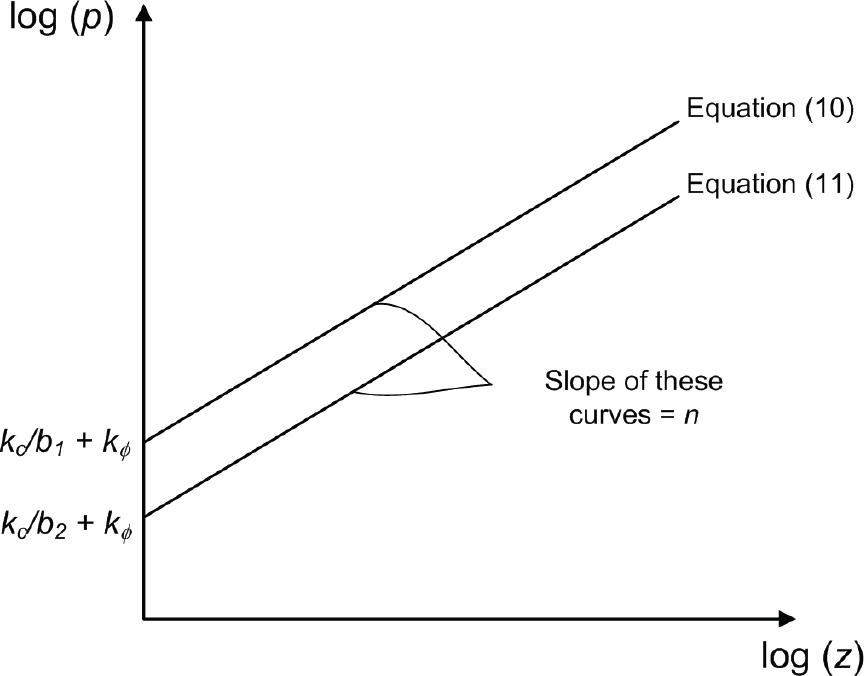
Pressure-sinkage curves for Equations (10) and (11)

The traditional way to carry out the pressure-sinkage experiment is to use a hydraulic system with pressure gauge installed (Bekker G., 1956), (Wong J.Y., 2001). However, due to high cost associated with the system, the Screw Press system is invented to acquire parameters k _c , k_φ, and n, Fig. 8.

Fig. 8.

Screw Press system developed for pressure-sinkage experiment, where, A is the screw press, B is the screw press's handle, C is the potentiometer fixed with the static part of the screw press, D is the experimental soil, E is the S-shape strain gauge, and F is the circular disc.

With the soil normal pressure (exerted from the disc) measured by the S-shape strain gauge (label E, Fig. 8) and the corresponding disc's sinkage measured by the potentiometer or linear position transducer (label C, Fig. 8), parameters k _c , k_φ, and n can be obtained by solving Equations (10) and (11).

5.3. Parameter K

Two methods described in (Wills B. M. D., 1963) are employed for measuring K. The first method uses annular torsional shear test (Hvorslev M. J., 1939). The apparatus for this test is driven by a hydraulic ram on an experimental soil. The values of applied torque and corresponding soil deformation are recorded using a special indicator and they are used for K calculation (Wills B. M. D., 1962). The second method involves using translational rigid track. The track is pulled by a hydraulic ram, and the shear force and corresponding soil deformation are measured from the oil pressure and movement of the piston, respectively (Wills B. M. D., 1962).

6. Experimental Results

In this section, the soil parameter identification results are presented based on experimental data taken from the test rig described in Section 4. From all the measured data obtained from experiments, the entire sets of measured DP, z, and i are used for soil parameter identification based on the algorithm developed in Section 3. There are 20 and 17 sets of data for Garside 60 soil and Garside iron sand respectively, acquired from wheel-terrain interaction test rig. The measured data for both soils were curve-fitted to a polynomial spline before being used as inputs to the algorithm. Tables 1 and 2 show the identification results for all 5 soil parameters for Garside 60 soil and Garside iron sand, respectively.

Table 1.

Identification results of 5 soil parameters for Garside 60 soil

Soil Parameters	Actual Values	Identified Value	Relative Error (%)
c (Pa)	0	62.52	N/A
φ (degree)	36	35.36	1.78
K (m)	0.01 – 0.025	0.01049	In range
S (N/mn+2)	199695.81	90416.37	54.72
n	0.71	0.53	25.35
Elapsed time (s)	0.344 (after 8 iterations)
DP prediction error (% rms)	7.25

Table 2.

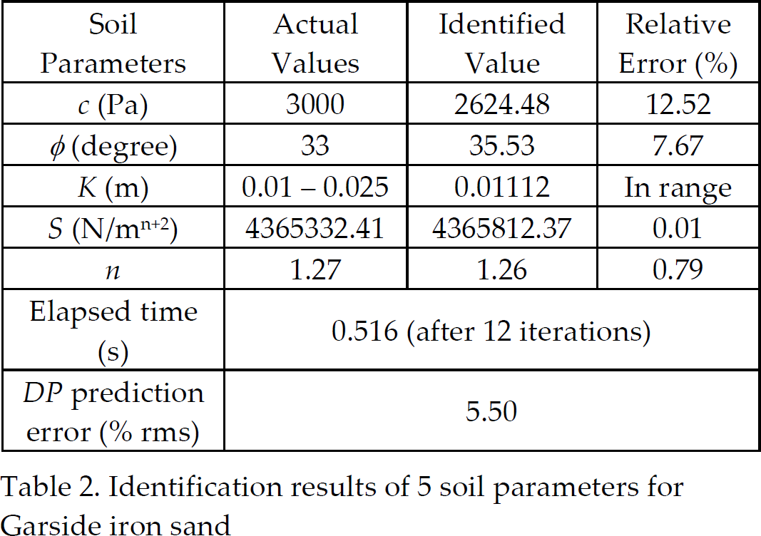
Identification results of 5 soil parameters for Garside iron sand

Soil Parameters	Actual Values	Identified Value	Relative Error (%)
c (Pa)	3000	2624.48	12.52
φ (degree)	33	35.53	7.67
K (m)	0.01 – 0.025	0.01112	In range
S (N/mn+2)	4365332.41	4365812.37	0.01
n	1.27	1.26	0.79
Elapsed time (s)	0.516 (after 12 iterations)
DP prediction error (% rms)	5.50

The identification algorithms were run on an Intel Pentium(R) 4 processor with a 2.80 GHz CPU and 1.00 GByte of RAM.

K varies from 0.01 m (firm sand) to 0.025 m (loose sand) for sand-like soils (Wong J.Y., 2001). The parameter K of both experimental soils falls within this range, as they are sands with varying degrees of compaction (firmness). In this study, since K is very difficult to measure and requires complex measuring devices (as described in Section 5.3), its value is assumed to be between 0.01 m and 0.025 m. Values of c and φ for both soils were obtained by the Direct Shear Test (Section 5.1), whereas their k _c , k_φ, and n were obtained from pressure-sinkage experiments (Section 5.2).

From Table 2 (using test rig data for Garside iron sand), the identification accuracies are relatively high with identification errors less than 12.52 % for all 5 parameters. For parameter K, ‘In range’ shown in percentage error column means that the identified K is within range of the actual K (0.01 m – 0.025 m). From Table 1 (for Garside 60 soil), the identification errors are quite high for parameters S and n (54.72 % and 25.35 %, respectively); however, they can be used to predict the drawbar pull with good accuracy (7.25 % rms error), Fig. 7 and Table 1. ‘N/A’ shown in percentage error column (Table 1) means that error for c cannot be computed since its actual value is equal to 0. However, its identified value is considered close to its actual value (the practical range of c for real-world soils is 0 Pa ≤ c ≤ 68500 Pa (Wong J.Y., 2001)).

Figures 9 and 10 are used to explain the reason for high identification errors of S and n. As illustrated in these figures, with a given set of values for c, φ, and K (c = 1000 Pa, φ = 34 degree, and K = 0.015 m), using different sets of values for S and n gives similar DP plots. When compared to the DP calculated using S = 500000 N/mⁿ⁺² and n = 0.64, the rms error of the DP calculated using S = 50000 N/mⁿ⁺² and n = 0.2 is 0.84 % (Fig. 9), while that of the DP calculated using S = 8800000 N/mⁿ⁺² and n = 1.2 is 1.15 % (Fig. 10). It can, therefore, be concluded that a slight deviation of DP inputs to the algorithm would yield different set of results for S and n. In reality, due to the random nature of the measurement noise, the measured DP will result in inaccuracies of identified pressure-sinkage parameters, S and n.

Fig. 9.

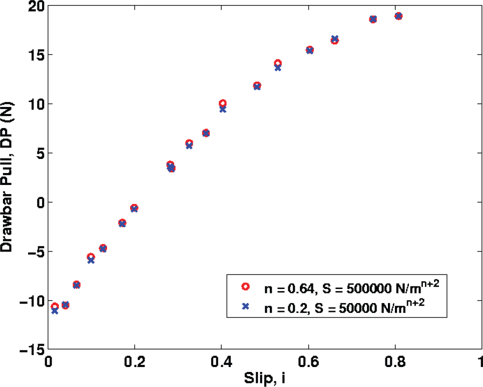
Plot of DP using c = 1000 Pa, φ = 34 degree, K = 0.015 m with different pairs of S and n (case 1 when using low-valued n)

Fig. 10.

Plot of DP using c = 1000 Pa, φ = 34 degree, K = 0.015 m with different pairs of S and n (case 2 when using high-valued n)

The identification times are 0.516 s and 0.344 s for Garside iron sand and Garside 60 soil, respectively. The execution time can be further reduced if the code is optimized. In this paper, the code is created using Matlab 6.5 running in command mode; the execution time can be significantly reduced, if an optimized code is executed. Therefore, the proposed algorithm has promising potential for on-line soil parameter identification for off-road wheeled vehicles.

The identification results from Tables 1 and 2 are used to predict the DP and compared with the experimental DP from the test rig, Figs. 11 and 12. From these figures, the rms errors are 7.25 % and 5.50 % for Garside 60 soil and Garside iron sand, respectively. This shows relatively good prediction accuracy of DP over the entire slip range using the identified soil parameters.

Fig. 11.

Comparison between the experimental DP and that predicted from the identified ‘c, φ, K, S, n’ for Garside 60 soil

Fig. 12.

Comparison between the experimental DP and that predicted from the identified ‘c, (, K, S, n’ for Garside iron sand

Next, a robustness test is carried out to examine whether the proposed algorithm will result in converged solutions when different initial conditions (p₀) are used. Table 3 gives the ranges of initial conditions that allow successful convergence. It is noted that values in brackets in this table are the practical range of parameters for real-world soils (Wong J.Y., 2001).

Table 3.

The range of initial estimates of soil parameters that produces the converged solutions for both experimental soils

Lower Bound	Soil Parameters	Upper Bound
0 (0)	c (Pa)	68500 (68500)
6 (6)	((degree)	40.1 (40.1)
0.006 (0.006)	K (m)	0.014 (0.05)
140000 (43720)	S (N/mn+2)	6321000 (6321000)
0.15 (0.11)	n	1.6 (1.6)

The algorithm shows good robustness to initial c and φ since any value chosen from their practical range results in converged solutions. However, for the other three parameters, it is recommended that initial K be chosen towards its practical lower bound (0.006 m ≤ K ≤ 0.014 m), initial S be chosen towards its practical upper bound (140000 N/mⁿ⁺² ≤ S ≤ 6321000 N/mⁿ⁺²) and initial n be chosen towards its practical upper bound (0.15 ≤ n ≤ 1.6). It is noted that the practical lower and upper limits of parameter S varies upon the wheel's width of the wheeled vehicle employed.

To sum up, by measuring DP and z samples at 5 or more slip values, soil parameters can be identified and used to predict the vehicle DP over the entire range of slips. These identified soil parameters can also be sent to following vehicles to improve their navigation on terrains ahead. Hence, accurate DP prediction of a wheeled vehicle over a particular terrain can be achieved. Consequently, based on accurate prediction of vehicle DP, the proposed algorithm can potentially be advantageous for traversability prediction and traction control for off-road wheeled vehicles.

6. Conclusions and Future Work

This paper investigates soil parameter identification for wheeled vehicles traversing unknown terrain based on a wheel-terrain interaction dynamic model and sensor feedback (drawbar pull, wheel slip, and wheel sinkage). The paper presents a new real-time approach for identifying all the unknown soil parameters required for drawbar pull prediction based on the Generalized Newton Raphson (GNR) method. This is the first time a technique for identifying all the unknown soil parameters for wheeled vehicles is proposed. The experimental data from the wheel-terrain interaction test rig are used to validate the feasibility and effectiveness of the approach. The results show that, despite high identification errors for some parameters, the identified soil parameters can be used to predict the drawbar pull with good accuracy. The range of initial estimates for each parameter that give converged solutions is also proposed. With terrain parameters identified by the proposed algorithm, the vehicle drawbar pull for off-road wheeled vehicles can be predicted for all driving conditions. The identified terrain parameters can also be forwarded to vehicles following behind to improve their navigation on that terrain. The technique can be applied to any wheeled vehicle with rigid wheels or deformable wheels with relatively high inflation pressure.

Future work will focus on the outdoor testing with a real wheeled vehicle or wheeled mobile robot.