Offensive Strategy in the 2D Soccer Simulation League Using Multi-Group Ant Colony Optimization

Abstract

The 2D soccer simulation league is one of the best test beds for the research of artificial intelligence (AI). It has achieved great successes in the domain of multi-agent cooperation and machine learning. However, the problem of integral offensive strategy has not been solved because of the dynamic and unpredictable nature of the environment. In this paper, we present a novel offensive strategy based on multi-group ant colony optimization (MACO-OS). The strategy uses the pheromone evaporation mechanism to count the preference value of each attack action in different environments, and saves the values of success rate and preference in an attack information tree in the background. The decision module of the attacker then selects the best attack action according to the preference value. The MACO-OS approach has been successfully implemented in our 2D soccer simulation team in RoboCup competitions. The experimental results have indicated that the agents developed with this strategy, along with related techniques, delivered outstanding performances.

1. Introduction

As one of oldest leagues in RoboCup, the 2D soccer simulation league has achieved great success and inspired many researchers all over the world to engage in this game each year [1]. Without the necessity to handle any low-level hardware problems, the 2D soccer simulation league focuses on high-level functions, such as cooperation and learning. Furthermore, the 2D soccer simulation league also provides an important experimental platform, which is a fully distributed, multi-agent stochastic domain with continuous state, action and observation space [2]. AI researchers have been using this platform to pursue research in a wide variety of domains, including cooperation, coordination and negotiation in real-time multi-agent systems.

As the environment of 2D soccer simulation is highly dynamic and unpredictable, it is very difficult to train agents' actions and generate a team strategy. Researchers have done a lot of work in this domain. Fang presented the Monte Carlo method to develop a team's defensive strategy [3]. Amir presented a reinforcement learning method to find a better way to dribble the ball and to break through opponents who are blocking the way to the goal [4]. Shi employed the Markov decision process to solve the proximal dribble problem [5]. Zhang presented a value strategy to improve the success rate of passing action [6]. Illobre used inductive logic programming to anticipate the shooting action of opponent players [7]. Cai employed mathematical analysis and a BP neural network to improve interception success probability [8]. Liu proposed a Support Vector Regression method to predict the distance that the ball will cover when the agent successfully intercepts the ball [9]. These methods have greatly improved the efficiency of the agent's actions. Given that the problem of multi-agent cooperation and the team's overall strategy has yet to be solved, this issue continues to provoke significant interest [10].

Using the powerful optimization capability of swarm intelligence methods, this paper presents an offensive strategy based on multi-group ant colony optimization (MACO-OS). Combined with the piecewise characteristics of attack action selection, the strategy algorithm dynamically selects the best attack action according to the real-time scene-information of the competition environment.

This paper is organized as follows: In section 2, we introduce the background to the 2D soccer simulation league. Section 3 introduces three primary attack actions and analyses the major influencing factors of these actions in the competition. Section 4 defines the parameters of ant colony optimization when it is applied to the offensive strategy in the RoboCup 2D soccer simulation league, as well as introduces MACO-OS in detail. In section 5, we run the algorithm on the RoboCup 2D soccer simulation league platform to verify the effectiveness of MACO-OS. Finally, section 6 concludes the paper with a discussion about future work.

2. Background

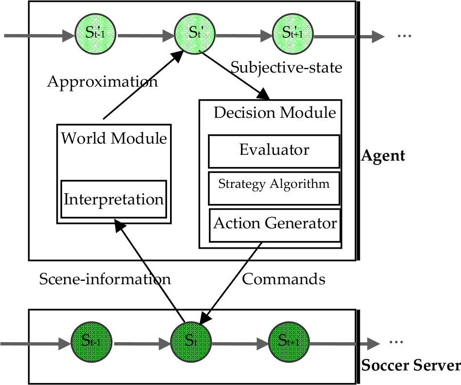
In the 2D soccer simulation league, a central soccer server simulates a two-dimensional virtual soccer field in real-time. Two teams of independently moving software players (called agents) connect to the server via network sockets in order to play soccer on a virtual field inside a computer [11]. Each team can have up to 12 clients including 11 players (10 fielders and one goalkeeper) and a coach. Each agent receives a set of scene-information (visual, acoustic and physical) from the soccer server, interprets this relative information and generates a world model with the interpretation module. The agent then selects an action and sends it to the server in real-time, with each of the agents having a chance to act 10 times per second. Each of these action chances is called a “cycle”. Visual information is sent six or seven times per second. During a standard 10-minute game, this gives 6,000 action chances and 4,000 receipts of visual information [12].

Based on the scene-information, each agent selects an action with the following steps: 1) evaluating the subjective state described in world model; 2) making a decision using the strategy algorithm; and 3) generating and refining basic commands (such as dashing in a given direction with certain power, turning the body or neck at an angle, kicking the ball at an angle with specified power, or slide-tackling the ball). The observation for each player contains noisy and local geometric information, such as the distance and angle to other players [13, 14], such that the state of the world model may have little deviation from that of the real world. The structure of the 2D soccer simulation is depicted below:

The task in the 2D soccer simulation league is to find the best action to execute from all possible world states (derived from the sensor input by calculating a sight on the world as absolute and noise-free as possible). Each agent has to interpret scene-information in a subjective state and select the best action to influence the environment. The state space and action space can be described as follows:

State space - A sequence of scene-information, observations, which include the current positions of the ball and all players (teammates and opponents), visions, physics and so on. The state of 2D soccer simulation can be represented as a fixed-length vector, containing state variables that totally cover 23 distinct objects (10 teammates, 11 opponents, the ball and the agent itself).

Action space - All actions that the agent may perform, i.e., shoot, pass, dribble, position, intercept, block, trap, mark and formation. The former three actions (shoot, pass, and dribble) belong to attack actions of the ball-handler, the last four actions (block, trap, mark, and formation) belong to defence actions, while the middle two actions (position, intercept) can be used in both attack and defence for the player without the ball. Each action is defined as follows [15]:

1. Shoot - to kick out the ball to score

2. Pass - to kick the ball to a proper teammate

3. Dribble - to take the ball forward with repeated slight touches or bounces in an appropriate direction

4. Position - to arrive in a particular place or manner to get a better chance of attacking or defending

5. Intercept - to get the ball as fast as possible

6. Block - to make the movement of an opponent (who controls the ball) difficult or impossible

7. Trap - to hassle the ball-handler and try to steal the ball

8. Mark - to be assigned to a specific opponent with the aim of denying them possession of the ball

9. Formation - how the players in a team are positioned for defence

The challenge in the 2D soccer simulation league comprises two aspects: the scene-information sent to each agent is relative and noisy, and the subsequent positions of every teammate and opponent are unpredictable because of the influences between agents.

3. Analysis of the main attack actions

In the 2D simulation league, there are three principal attack actions in relation to the ball-handler: shoot, pass and dribble. In this section, we analyse the main factors of each action and, in turn, create appropriate models.

3.1. Shooting model

The shooting point must fulfil two main conditions: 1) it must be in the area of the goal, and 2) the goalkeeper and defender cannot intercept the ball. As shown in Figure 2, if we define the attacker as a vertex, there will be several angles made by the defenders, goalkeeper and goalposts. The best angle is the maximum angle (called the gap angle), and the best shooting point is the bisector neutral point of the gap angle. The distance between the attacker and the goal is called the shooting distance. It is obvious that there is a strong correlation between shooting success and the neutral point of the gap angle. The greater the gap angle, the shorter the shooting distance and the higher the shooting hit rate. The gap angle and shooting distance are denoted as α _shoot and d _shoot , respectively.

Figure 1.

Structure of 2D soccer simulation

Figure 2.

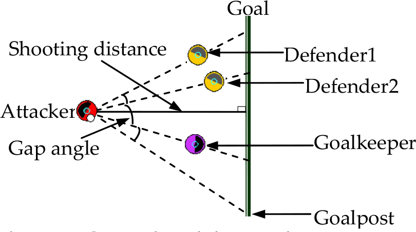
Gap angle and shooting distance

3.2. Passing model

In order to change the attack azimuth quickly, the attacker must pass the ball to his teammate. The passing target point may be the position where the teammate stands, or the space behind the defenders. Before passing the ball, the attacker needs to predict whether the defender will catch the ball when it is passed in a certain direction. The success ratio is calculated by comparing the time taken for the ball and the defender to reach the cut-off point. According to this success ratio, the attacker can select a prime passing direction and determine whether to pass or not. As shown in Figure 3, the time taken for the ball and the defender to reach the cut-off point is determined once the intercept distance and passing angles are also determined. Thus, we look to passing angles and intercept distance as the major factors. For convenience, the passing angles and intercept distance are denoted as α _pass and d _intp , respectively.

Figure 3.

Intercept distance and passing angles

3.3. Dribbling model

In order to increase the dribbling speed, we do not require the ball to be in the control of the attacker when he is in the penalty area. The agent may kick the ball away in a certain range, which may be beyond the control of the agent, and then use intercept technology to catch the ball before the defender does. This method needs to consider the attacker's dribbling distance and the defender's intercept distance after two cycles or longer, which is denoted as d _drib and d _intd , respectively. A diagram of the dribbling model is shown in Figure 4.

Figure 4.

Dribbling distance and intercept distance

4. Offensive strategy algorithms

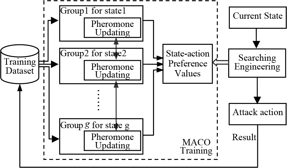
In the 2D soccer simulation league, the field state has many properties describing offence and defence, such as the relative positions, the distance from the ball, the members in a certain region and so on. It is easy to see that the field state is a continuous space. To deal with the state data quickly and effectively, we need to divide them into many equivalent states by a process of discretization. In the course of a soccer game, the attacking strategy varies with the state. That is to say, attacking strategy is a piecewise function: the best attack action may be different if the field state changes. Furthermore, we must identify the best action for each state. In this paper, we set a path for each action in each state, and found the best action in a given state via the preferences of the paths. According to the theory of ACO, we should regard each attack action as a path in the solution space, consider each agent's training in the same way we would foraging behaviour of an ant, and treat an effective attack as success foraging. In order to solve the problem of “a solution per state”, we set an ant group for each equivalent state (an equivalent state is considered as an interval in the piecewise function) for the purposes of this paper. Within this setting, each ant lays down a trail pheromones on a path (corresponding to the preference value of an attack action), and each ant group may have a path that has the highest pheromone level (corresponding to the best preference value and the best attack action). Hence, we could get the best preference values for every state via the multiple ant groups. For this paper, an action training algorithm was devised based on multi-group ant colony optimization [16]. The algorithm created an ant group for each state, interacted pheromones with similar groups and produced a data set to save the preference values of actions for every state. Using the method of increasing the pheromone mechanism of ACO, the algorithm formed a mechanism of positive feedback between action affection and pheromones. In the process of the 2D soccer simulation competition, the agent receives a set of scene-information (visual, acoustic and physical) and translates this information into equivalent states. The agent then searches the data set of the state-action preference values, selecting an action that has the most similar state and the highest preference value. Finally, the agent makes the selected action, evaluates the result of the action after a given time (set as five cycles in this paper) and sends the result to the training data set as a new sample. The flowsheet of action training and selection is demonstrated below:

According to the parameters, such as pheromone level, the value for each state could be calculated, while the best attacking strategy could be selected for each state. To avoid the problem of a state of sparseness, we created an Attack Information Tree (which will be described fully in subsection 4.2) to update the pheromones in real time. Thus, the offensive strategy we selected has a dynamic character. Subsection 4.1 will describe the main parameters of MACO.

4.1. Parameters of MACO

By depicting attack actions as paths of foraging, parameters (pheromone level, heuristic information and preference function) are defined as follows:

Definition 1 - Pheromone level (denoted as τ _k ^l (t)) represents the intention of the k-th group ants to choose path l, which decreases with time and increases with the ants' success on path l.

${\tau }_k{}^{l\hspace{0.17em}}\left(t+1\right)\hspace{0.17em}=\hspace{0.17em}\left(1-\rho \right){\tau }_k{}^l\left(t\right)\hspace{0.17em}+\delta \hspace{1em}{\tau }_k{}^l\hspace{0.17em}$

(1)

where ρ is the coefficient of pheromone evaporation, δ is the constant associated with the pheromone level, and $\Delta {\tau }_k{}^l$ refers to the added pheromones of ants in the k-th group on path l.

$\hspace{1em}{\tau }_k{}^l={\displaystyle {\sum }_{i=1}^{m_k}\hspace{1em}{\tau }_{k,i}{}^l}$

(2)

where m _k is the ant number of the k-th group, and $\Delta {\tau }_{k,i}{}^l$ refers to the added pheromones on path l by the i-th ant in k-th group.

$\hspace{1em}{\tau }_{k,i}{}^{l\hspace{0.17em}}=\{\begin{array}{l}\begin{array}{ccc}1& & \text{Success}\end{array}\\ \begin{array}{ccc}0& & \text{Failure}\end{array}\end{array}$

(3)

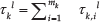
where the success and failure are foraging results on the path l (each path corresponds to an action in a state), respectively. If an action has achieved the expectation of its executive agent (e.g., the passing agent expects that the target teammate will get the ball, and the shooting agent wants to score), we call it “success”; otherwise, we call it “failure”.

Definition 2 - Heuristic information (denoted as η _k ^l) is the experience of ants in the k-th group to choose the path l (corresponding to the l-th attack action selected by agent), and η _k ^l may be expressed by the access frequency of path l.

${\eta }_k{}^l=\frac{C_k{}^l}{{\displaystyle {\sum }_{i=1}^n{C}_k{}^i}}$

(4)

where n is the total number of paths, and C _k ^l is the access number of ants in the k-th group on path l.

Definition 3 - Group similarity (denoted as S _k,j ) is the similarity degree between two groups, which may be calculated by the similarities of the field states of the two groups (k and j). Suppose that f is a h-dimensional vector, f _k is the field state (including various relative distances and angles amongst offence, defence and the ball, such as αshoot, dshoot, αpass) of the group k, and f_k,i is the i-th dimension of f _k , then the value of S _k,i is:

$S_{k,i}\hspace{0.17em}=\frac{1}{h}{\displaystyle {\sum }_{i=1}^h{\left(f_{k,i}-f_{j,i}\right)}^2}$

(5)

When an ant finds an optimum solution, it will share its solution with similar groups, which have the minimum value of S _k,i . For example, when an ant from the k-th group learns a success action, it will add pheromones to its own path (as described in Definition 1), and also add pheromones to similar groups (denoted as SG). Given that the group number of SG is g, the pheromones of each group in SG may be added as:

${\tau }_i{}^{l\hspace{0.17em}}\left(t\right)\hspace{0.17em}={\tau }_i{}^{l\hspace{0.17em}}\left(t\right)\hspace{0.17em}+\hspace{1em}{\tau }_k{}^{l\hspace{0.17em}}$

(6)

Definition 4 - Preference function (denoted as $p_k^{l,i}\left(t\right)\hspace{0.17em}$ ) is the tendency of the i-th ant in the k-th group to choose path l, which is affected by pheromones ${\tau }_k^l\left(t\right)$ and heuristics (η _k ^l ). The expression of preference function is defined as:

$p_k^{l,i}\left(t\right)\hspace{0.17em}=\frac{{\left[{\tau }_k^l\left(t\right)\right]}^{\alpha }\cdot {\left[{\eta }_k^l\right]}^{\beta }}{{\displaystyle \sum _{j=1}^n{\left[{\tau }_k^l\left(t\right)\right]}^{\alpha }\cdot {\left[{\eta }_k^l\right]}^{\beta }}}$

(7)

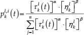
where α, β are the adjustment factors of pheromones and heuristics, respectively. In the case of ignoring heuristic information, the value of β may be zero. According to the value of $p_k^{l,i}\left(t\right)\hspace{0.17em}$ , which may be calculated by Equation 7, we can achieve the best attack action for the current field environment.

4.2. Offensive strategy algorithm based on MACO

We can simulate different attacking environment by setting agents at different points on the field. Regarding three attack actions (shooting, passing and dribbling) as three different paths for foraging, we can obtain the best attack action by using the preference values of ants' foraging behaviours. The following two steps should be made in order to find the best attack action: 1) train the preference values of actions in each environment, and 2) select the best attack action based on preference value. The first step runs offline in the background for a long time to obtain the preference value; the second step is designed using the decision module of the attacker and runs online to select the best action.

The state of attacking environment is a continuous space. In order to deal with the state data quickly and effectively, we should transfer them into many discrete equivalent states. The discretization function is defined as:

$x_i^{’}=\{\begin{array}{l}Truncate(x_i/\hspace{0.17em}(Max\left(i\right)/T)+1\hspace{0.17em})\hspace{0.17em}\hspace{0.17em}\hspace{0.17em}\hspace{0.17em}\hspace{0.17em}\hspace{0.17em}\hspace{0.17em}\hspace{0.17em}\hspace{0.17em}\hspace{0.17em}\hspace{0.17em}\hspace{0.17em}{x}_i\hspace{0.17em}(T-1)*(Max\left(i\right)/T)\hfill \\ T\hspace{0.17em}\hspace{0.17em}\hspace{0.17em}\hspace{0.17em}\hspace{0.17em}\hspace{0.17em}\hspace{0.17em}\hspace{0.17em}\hspace{0.17em}\hspace{0.17em}\hspace{0.17em}\hspace{0.17em}\hspace{0.17em}\hspace{0.17em}\hspace{0.17em}\hspace{0.17em}\hspace{0.17em}\hspace{0.17em}\hspace{0.17em}\hspace{0.17em}\hspace{0.17em}\hspace{0.17em}\hspace{0.17em}\hspace{0.17em}\hspace{0.17em}\hspace{0.17em}\hspace{0.17em}\hspace{0.17em}\hspace{0.17em}\hspace{0.17em}\hspace{0.17em}\hspace{0.17em}\hspace{0.17em}\hspace{0.17em}\hspace{0.17em}\hspace{0.17em}\hspace{0.17em}\hspace{0.17em}\hspace{0.17em}\hspace{0.17em}\hspace{0.17em}\hspace{0.17em}\hspace{0.17em}\hspace{0.17em}\hspace{0.17em}\hspace{0.17em}\hspace{0.17em}\hspace{0.17em}\hspace{0.17em}\hspace{0.17em}\hspace{0.17em}\hspace{0.17em}\hspace{0.17em}\hspace{0.17em}\hspace{0.17em}\hspace{0.17em}\hspace{0.17em}\hspace{0.17em}\hspace{0.17em}\hspace{0.17em}\hspace{0.17em}\hspace{0.17em}\hspace{0.17em}\hspace{0.17em}\hspace{0.17em}\hspace{0.17em}\hspace{0.17em}\hspace{0.17em}\hspace{0.17em}\hspace{0.17em}\hspace{0.17em}\hspace{0.17em}\hspace{0.17em}\hspace{0.17em}\hspace{0.17em}\hspace{0.17em}\hspace{0.17em}\hspace{0.17em}\hspace{0.17em}\hspace{0.17em}\hspace{0.17em}\hspace{1em}\hspace{1em}\hspace{0.17em}\hspace{0.17em}\hspace{0.17em}{x}_i\ge (T-1)*\hspace{0.17em}(Max\left(i\right)/T)\hfill \end{array}$

(8)

where T is the equivalent state number of each state in the discretization process (interval number), and Max(i) is the original maximum of state data x _i .

The format of training data is (αshoot, dshoot, αpass, dintp, ddrib, dintd, aa, suc), where aa is attack action and suc is the result of the attack action (failure: 0, success: 1). Assuming that the maximum for each state (αshoot, dshoot, αpass, dintp, ddrib, dintd) is defined as (π, 30, π, 30, 3, 3), respectively, and the equivalent state number of each state (T) is defined as 10, then the data (0.6, 11.5, 0.5, 3.6, 0.9, 1.2, shooting, 1) will be discretized as (2, 4, 2, 2, 3, 4, 1, 1), according to Equation 8. Likewise, the data (0.2, 14.3, 0.3, 1.7, 0.7, 0.8, passing, 0) will be discretized as (1, 5, 1, 1, 3, 3, 2, 0).

In order to save the success rate and the preference values of the three attack actions for each state, we created an Attack Information Tree (AIT), based on a multi-branch tree model (as shown in Figure 6). For example, the discretized data (2, 4, 2, 2, 3, 4, 1, 1) are stored in the Node ₂₄ (the leaf on the path whose αshoot=2 and dshoot=4) of the first tree (root ₁ ), because the value of (αshoot, dshoot, aa) is (2,4,1). Likewise, the data (1, 5, 1, 1, 3, 3, 2, 0) are stored in the Node ₁₁ of the second tree (root ₂ ), because the value of (αpass, dintpt, aa) is (1,1,2). Each leaf of the tree has four-dimensional data (fail:int, succ:int, sucRate:float, preference:float), where fail is the amount of failure, succ is the amount of success, sucRate is the success rate counted by τ _k ^l (t), and preference is the preference value denoted as p _k ^l,i (t), as per Definition 6.

Figure 5.

The flow sheet of action training and selection

Figure 6.

The structure of the Attack Information Tree for three actions

For every attacking environment (state), we generated a group of ants and used pheromone concentration to record the dynamic success-rate of each attack action. When we obtained training data, we counted the pheromone level and heuristic information using Equations 1–4. According to the ant colony algorithm, the preference value p _k ^l,i (t) can be counted using Equation 7. Based on multi-group ant colony optimization, the algorithm for training with regard to the AIT (MACO-AIT) is as follows:

Algorithm-1.

MACO-AIT algorithm

Input: Pre-processed training data set D (m records) Output: Attack Information Tree (AIT) Step 1: Initialize, Tree _shoot = Tree _pass = Tree _drib = NULL; AIT={Tree _shoot , Tree _pass , Tree _drib }; Step 2: FOR (i=1 to m) Find the Tree in AIT by aa of the i-th record; Seek i-th record in the Tree; IF found THEN Update τ ^l _k (t) by Definition 1; Update C ^l _k by Definition 2; Find similar groups by Eq. 5 and save in SG; FOR each group in SG Update τ ^l _i (t) by Equation 6; ENDFOR ELSE Create a sub-tree for remaining parameters; Initialize the value of C ^l _k , τ ^l _k (t); Link the new sub-tree to its parent node; ENDIF ENDFOR Step 3: Calculate η ^l _k for every leaf by Equation 4; Step 4: Initialize the adjustment factors (α,β); Initialize the preference function p^l,i_k(t); FOR each Tree in AIT FOR each path l in the Tree Calculate the value of p^l_k (t) by Equation 7; Save p^l_k(t) to preference of the leaf on path l; ENDFOR ENDFOR Step 5: RETURN AIT;

Step 4 initializes the adjustment of pheromone (α) and heuristic (β) factors. Under normal conditions, the reasonable definition ranges are: α∈[0, 2], β∈[1, 10] (we set α=2, β=4, respectively, in this paper).

For a specific state, the fitness level of the attack action is positively related to its preference value. The most appropriate action will have the highest preference value in training. Therefore, we can find the most appropriate action via the preference value. Using the AIT trained by multi-group ant colony optimization, we can search the state in every tree in the AIT and obtain the preference values of every attack action. In turn, the maximum preference value (corresponding to the best attack action to current state) should be selected. The MACO-OS algorithm is as follows:

Algorithm-2.

OS algorithm

Input: Discretized real-time field data (X), trained AIT Output: Attack action (act) Step 1: Load AIT trained by MACO-AIT algorithm; Initialize, pref = bstpref = 0, fail=thefail=0, act = random(action_list); Step 2: FOR each tree in AIT Find the path l corresponding to X; IF found THEN pref =l.preference; fail =l. fail; ELSE Find two paths l₁,l₂ closest to X; pref =(l₁.preference+l₂.preference)/2; fail =(l₁. fail+l₂. fail)/2; ENDIF IF pref > bstpref THEN bstpref = pref; thefail= fail; act =this.action; ENDIF ENDFOR Step 3: IF bstpref < threshold AND actfail >1 THEN act =back-pass; ENDIF Step 4: RETURN act;

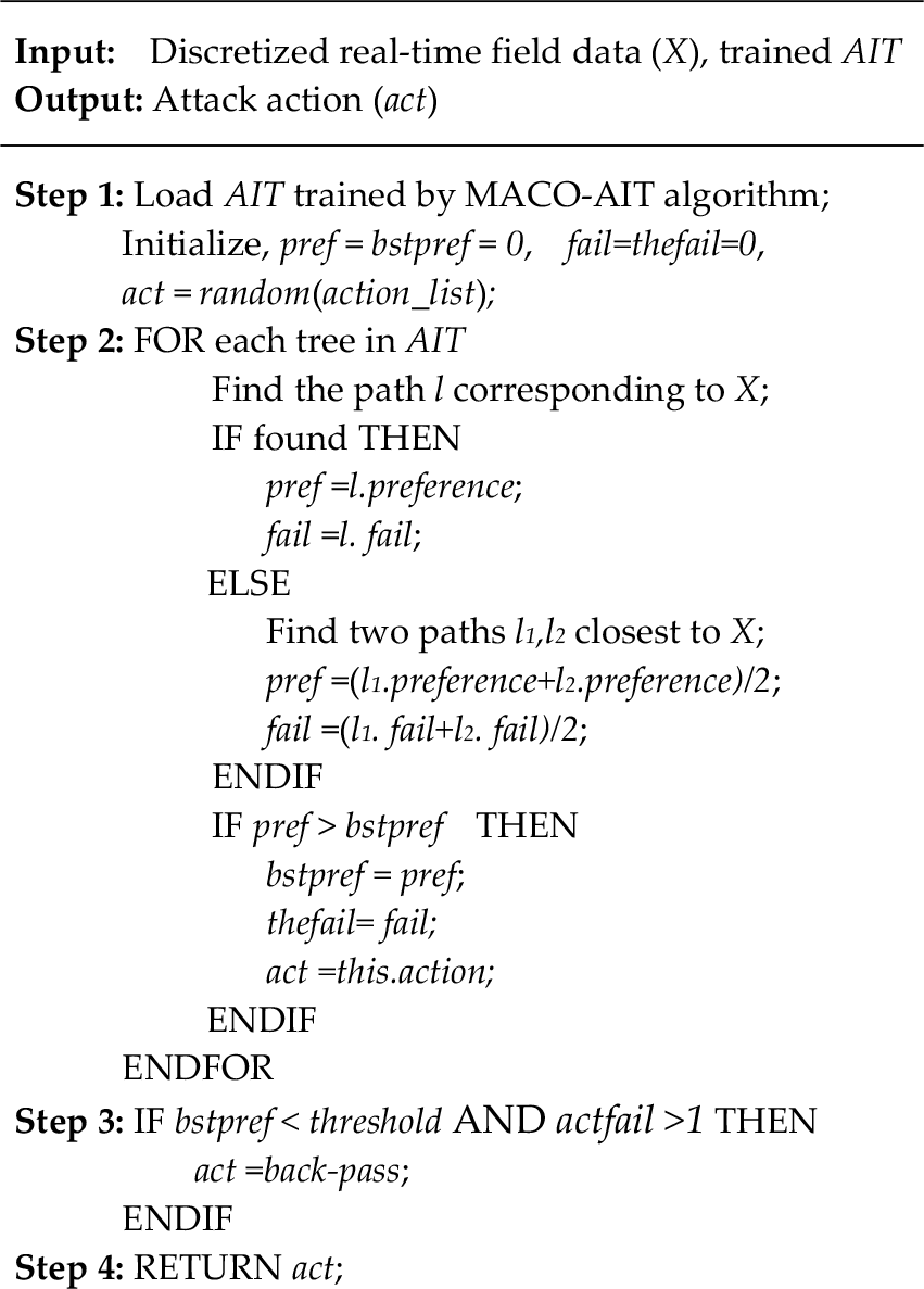
Step 2 searches data X in the AIT and results in the best attack action. If there is no path matched with X, the algorithm will find the two closest paths to X by Euclidean distance in the tree and obtain the average preference value of these paths. If there are three or more paths with the same smallest distance, the algorithm will select two of them randomly as the two closest paths. For a trained AIT, the preference of each leaf is not less than zero. Therefore, Step 2 can identify an action whose preference has the biggest value in the current state or the similar states. In Step 3, while all of the preference values of attack actions are rather low, the algorithm will select back-pass action, which passes the ball backwards. The reason is that all of attack actions would not have good preferences in this case. According to competition experiences, this is because the defence is very crowded. Therefore, we should pass the ball backwards to disperse defenders, then attack it again when the chance arises.

The space complexity of Algorithm-1 and Algorithm-2 are both O(s), where s is the size of the AIT. Supposing each state data are discretized into T elements, the size of the AIT (s) should be O(3*T²⁾. The time complexities of Algorithm-1 and Algorithm-2 are O(I *n^2*m*g*lg(g)) and O(n*lg(g)), respectively, where n, g, m, I are the number of actions, groups, ants and iterations, also respectively. Algorithm-1 seems to have a high time complexity. But, in the case of attack action selection, n is equal to 3 (action number) and (I*m) is equal to the training times. Therefore, Algorithm-1 should run well in a practical application.

5. Experimental evaluation

After being created, the 2D soccer simulation team with the MACO-OS was run in the RoboCup simulation platform to evaluate our new algorithm. Firstly, every agent took random attack actions. The results of these actions have been recorded and used for the next training session. The underlying code and underlying database are Agent2d-3.1.1 and Librcsc, respectively. The positions of all players (two attackers, two defenders and one goalkeeper) were set randomly by an offline coach. After five cycles of competition, the results of two teams are recorded as the format of “αshoot, dshoot, αpass, dintp, d_drib, dintd, aa, suc”. The training will stop after 150,000 times. The training scene is shown in Figure 7. In order to show the situations of the attack and defence sides more clearly, only the penalty area is depicted.

Figure 7.

Screenshot of training scene arranged randomly

In the following experiments, the maximum value for each state data (αshoot, dshoot, αpass, dintp, ddrib, dintd) was defined as (π/2, 15, π/2, 15, 3, 3), respectively, with each state discretized into 30 elements. If state data are larger than the defined maximum, the discretized data will be the maximum value according to the Equation 8 (e.g., if the value of αshoot is equal to 2π/3, then the discretized value of αshoot will be 30). The number of states was 2,700 (3*30 ² ), the number of groups was 2,700 and the number of ants was 8,100 in total. The adjustment factors for pheromones and heuristics were set as follows: α=2, β=4. In order to keep the previous experiences obtained during the pre-event training, we set the coefficient of pheromone evaporation at a low level (ρ=0.1). All of experiments ran on the same computer (memory: DDR3 8G, CPU: i5-4570).

5.1. An example of an attack process

In order to illustrate the application of the AIT, a simplified example of an attack process is described in this section. Firstly, we trained the record data and obtained AIT by multi-group ant colony optimization. Then, the MACO-OS algorithm was used in the attacker decision module. In a simulation of the common attacking environment, we placed two attackers, two defenders and one goalkeeper. The attack process is depicted in Figure 8 (a, b, c, and d): two attackers (No. 9 and No. 10) have selected three attack actions (passing, dribbling and shooting), according to the AIT and scene-information. Here, we assume that the first action selection starts at t₀ cycle.

Figure 8.

An example of an attack process using the AIT

In this example, the ball-handler selects the action that has the maximal preference value of path l in the AIT (which consists of three trees named passing, dribbling and shooting). The path l corresponds to the scene-information, while the value of preference is counted by the success times of the action in training.

5.2. Competitions with baseline strategy

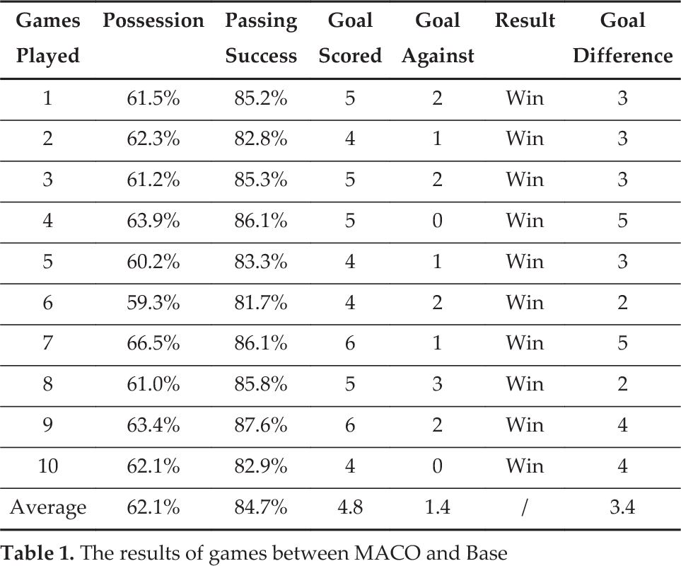
Application effect in competition is the sole criterion for evaluating an offensive strategy. This section concerns our creation of a 2D soccer team named MACO, which employs the MACO-OS algorithm as the offensive strategy. Meanwhile, using the underlying code Agent2d-3.1.1, which is an open source by Helios (former world champion in the RoboCup 2D simulation league), we created another team (named the BASE team), which adopted the searching-space offensive strategy. The only difference between the MACO team and the BASE team is the attacking selection strategy. There were 10 games in total in the test, with each game running 6,000 standard clock cycles. The results of the games are presented below:

As listed in Table 1, the MACO team dominated in the games with 62.1% possession and 84.7% passing-success on average. As a result, the MACO team enjoyed a 100% winning advantage with 3.4 goal differences per game, as well as scoring three times as many goals as its opponent on average.

Table 1.

The results of games between MACO and Base

Games Played	Possession	Passing Success	Goal Scored	Goal Against	Result	Goal Difference
1	61.5%	85.2%	5	2	Win	3
2	62.3%	82.8%	4	1	Win	3
3	61.2%	85.3%	5	2	Win	3
4	63.9%	86.1%	5	0	Win	5
5	60.2%	83.3%	4	1	Win	3
6	59.3%	81.7%	4	2	Win	2
7	66.5%	86.1%	6	1	Win	5
8	61.0%	85.8%	5	3	Win	2
9	63.4%	87.6%	6	2	Win	4
10	62.1%	82.9%	4	0	Win	4
Average	62.1%	84.7%	4.8	1.4	/	3.4

5.3. Competitions with other strategies

In recent Robocup 2D soccer simulation leagues, there have been two popular offensive strategies: the Value strategy and the Reinforcement Learning approach. Most of the top teams have used them or their variants, and have secured good results in turn. For this experiment, we created two 2D soccer teams (named the V team and the RL team):

V team - The Value strategy was employed to select the attack action. The field was divided into many small regions, which were assigned a value according to the threat of each region. A BP-neural network was trained to calculate the value of each action to a region, so that the attack action could be selected based on its value and the success probability.

RL team - The Reinforcement Learning approach was used to select the attack action. A binary search tree (BST) was created to save the information of the states, the actions and the values of rewards. At each time t, the agent received an observation o_t from the world model, with which we estimated the values of reward r_t using the following two steps [11, 15]: 1) calculating the heuristic-value of the state (v_t) by the observation o_t (which includes ball position, teammates, opponents and ball speed); and 2) assigning value to r_t by the difference between v_t and v_t-1. The agent was then able to find its former states in BST and added r_t to it. According to the BST value, the agent selected an action a_t, which was subsequently sent to the server and affected the environment. The environment then moved to a new state s_t+1.

We created two teams, which respectively used the Value strategy and the Reinforcement Learning approach as the offensive strategy. The other modules of these teams used the same code as the MACO team described in subsection 5.2. Moreover, all of teams (the V team, the RL team and the MACO team) possess the same training samples and the same training times, and run on the same computer (having the same memory capacity and computing capability). The MACO team played five games with the V team and the RL team, respectively. The results of each game are as follows:

In Table 2, GS, GA and GD respectively denote goal scored, goal against and goal difference. In order to analyse the performance of the MACO team, a sign test was introduced. First, we selected the sign for each game (‘+’ for win, ‘#’ for draw and ‘−’ for loss). Then, the number for each sign was calculated as follows:

Table 2.

The results of games between different teams

Games Played	MACO vs V					MACO vs RL
	1	2	3	4	5	1	2	3	4	5
GS	2	3	3	2	3	3	3	4	2	4
GA	1	1	2	2	1	3	2	3	2	3
GD	1	2	1	0	2	0	1	1	0	1
Result	win	win	win	draw	win	draw	win	win	draw	win

Table 3 describes the sign of each game. Suppose n₊, n- is the total of sign ‘+’ and sign ‘−’, respectively, and N is the sample size excluding ties between the samples, the sign tests are taken as follows:

Table 3.

The signs for the games between different teams

Games Played		1	2	3	4	5	Total
							+	−
MACO vs. V	GD	1	2	1	0	2
	Sign	+	+	+	#	+	4	0
MACO vs. RL	GD	0	1	1	0	1
	Sign	#	+	+	#	+	3	0

First, we tested the results of the games between the MACO team and the V team. Table 3 shows that n₊=4, n-=0, then N=n₊+n-=4, r=Min(n₊, n-)=0. According to the critical values of the sign test, r≤r_0.01. Hence, the MACO team is better than the V team at a significance level of 0.01.

Likewise, having tested the results of the games between MACO and RL in Table 3, we can also conclude that the former is better than the latter also at a significance level of 0.01.

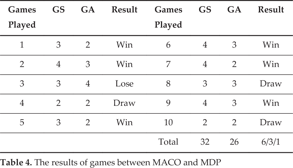
In order to enable the MACO-OS to compete more strategically, we created another 2D soccer team, named the MDP team, and was developed based on the Markov Decision Processes (MDP), which was used by the WrightEagle team (a five-time world champion in the 2D league). Compared to the RL team, the MDP team uses the searching forward approach to select the best action. Firstly, a binary search tree (BST) was created to record the information of states, states values (SV), actions, expected actions values (AV) and transitions probabilities (TP). Then, for a state s, the agent computed AV and TP of each possible action by searching forward in BST. According to paper [15], the search in BST is processed in a depth-first fashion until a goal state or a certain pre-determined fixed depth is reached. When it reached the depth, the heuristic-values of SV were evaluated and sent to state s as the long term value of AV [15]. With the same memory capacity and computing capability, the MACO team played 10 games with the MDP team. The results of these games are presented below:

Table 4 shows that the MACO team performed better than the MDP team, with six wins, three draws and one loss. This indicates that the MACO team has a 75% chance of beating the MDP team, which is satisfying since the environment is unpredictable, while the action may sometimes be affected by accidental factors. As far as action selection is concerned, the MACO-OS algorithm performed better than the MDP algorithm. This is because the MDP algorithm uses the searching forward approach, which needs a great deal of memory and computing time.

Table 4.

The results of games between MACO and MDP

Games Played	GS	GA	Result	Games Played	GS	GA	Result
1	3	2	Win	6	4	3	Win
2	4	3	Win	7	4	2	Win
3	3	4	Lose	8	3	3	Draw
4	2	2	Draw	9	4	3	Win
5	3	2	Win	10	2	2	Draw
				Total	32	26	6/3/1

5.4. The scale of training times

In this stage, we analysed the training scale by simulations. The team described in the above experiments was trained 150,000 times. Had the team had been trained only a few hundred times, the result may have been quite different. In order to identify the appropriate range of training times, we used a different scale of training data and tested the effect of the corresponding AIT.

Firstly, we divided the training data collected using the above experiments into 10 parts, denoted as d₁, d₂,…, d₁₀, and set T_i = ${\displaystyle {\sum }_{k=1}^j{d}_k}$ to create 10 training data sets with different scales. Then, using the MACO-AIT algorithm to train those 10 data sets, AITs were generated and 10 teams created corresponding to these AITs. Meanwhile, after creating the previously mentioned BASE team, we made it compete 10 times with each of the 10 teams described above, respectively. The losing percentage, the drawing percentage, the winning percentage and goal difference on average are presented below:

Figure 9 shows that the winning percentage and goal difference are increased gradually with the increasing scale of the training in the early stages. However, when the training scale reached T₉, the winning percentage and goal difference reached the highest level. Besides, the losing percentage and the drawing percentage both reach zero, the lowest level. It can be concluded that the offensive strategy will mature after about 135,000 training times when each state is discretized into 30 elements (there were 2,700 states in total).

Figure 9.

The curve of result varied with the training scale when the equivalent state number of each state (T) is 30 (2,700 states in total)

In order to test whether the state number has an influence on the scale of training time, we discretized each state into 25 elements (there were 1,875 [3*25 ² ] states in total), and generated new training recorders whose format was also “αshoot, dshoot, αpass, dintp, d_drib, dintd, aa, suc”. Using the same method described at the beginning of this subsection, we then created 10 training data sets (T_i = ${\displaystyle {\sum }_{k=1}^j{d}_k}$ ), trained 10 AITs with these 10 data sets and created 10 teams with these AITs. Finally, we created the BASE team and played 10 games with each of the above 10 teams, respectively. The winning percentage and goal difference on average are presented below:

Figure 10 shows that the winning percentage and goal difference reached the highest level when the training scale reached T₆ (90,000 training times). Comparing Figure 10 with Figure 9, we found that the winning percentage and goal difference matured faster when the state number of training data got smaller. In order to verify this conclusion, we conducted experiments with other training scales. Setting the equivalent state number of each state (T) at 20 (1200 states), the winning percentage reached the highest level when the training scale was greater than T₄ (60,000 training times). From these, we were able to conclude that the offensive strategy will mature after about 50*3*T² training times.

Figure 10.

The curve of result varied with the training scale when the equivalent state number of each state (T) is 25 (1,875 states)

6. Conclusions

The offensive strategy is an important factor in the attacking capability of a soccer team. Given the unpredictability of the environment and the influence amongst agents, it is very difficult to select action for the ball-handler. Attacking strategy has becomes a hotly discussed issue in the domain of multi-agent cooperation in a real-time, asynchronous and noisy environment. In this paper, we analysed the principal factors of the main attack actions for the ball-handler in the 2D simulation league and presented a novel offensive strategy algorithm based on multi-group ant colony optimization (MACO-OS) in order to improve attacking efficiency. Using the pheromone evaporation mechanism, the algorithm creates an AIT, which is the basis of decision-making action. The MACO-OS algorithm has been implemented in our RoboCup 2D soccer simulation team (named MT2014), which has since won first prize in the 2014 China Open competition. However, the RoboCup 2D soccer simulation league is a multiple technologies competition, which includes offensive strategy, defensive strategy and defence conversion strategy. Our future work will focus on defensive strategy and defence conversion strategy to enhance the team's overall performance.