Sage Journals: Discover world-class research

Abstract

In this study, a method for the generation of tracking trajectory points, detection and positioning of obstacles in agricultural fields have been presented. Our principal contribution is to produce traceable GPS trajectories for agricultural vehicles to be utilized by path planning algorithms, rather than a new path planning algorithm. The proposed system works with minimal initialization requirements, specifically, a single geographical coordinate entry of an agricultural field. The automation of agricultural plantation requires many aspects to be addressed, many of which have been covered in previous studies. Depending on the type of crop, different agricultural vehicles may be used in the field. However, regardless of their application, they all follow a specified trajectory in the field. This study takes advantage of satellite images for the detection and positioning of obstacles, and the generation of GPS trajectories in the agricultural realm. A set of image processing techniques is applied in Matlab for detection and positioning.

Keywords

Autonomous Vehicles Labelling Obstacle Detection Image Processing Field Robotics

1. Introduction

Rapid developments in computational intelligence, which are parallel to developments in digital science and technology, launched a new age for the automation of traditionally manual industries including agricultural production. Higher quality and volume in agricultural production requires a higher efficiency in ploughing, seeding, harvesting and similar traditionally manual tasks [40]. Various types of automated agricultural vehicles may be needed and implemented, requiring the tracking of a specific trajectory in the field.

Studies on the low-level control of autonomous vehicles propose several methods to track with a sufficiently low lateral error [29, 24]. A higher level of agricultural automation requires the automatic preparation of the reference paths to be followed by autonomous agricultural vehicles. Path planning algorithms, which are based on splitting a field into trapezoidal subfields and merging them into larger blocks to solve routing by a straight line, is covered by [39]. Path planning algorithms based on level set methods are analysed in [5] to improve re-computations in the case of environmental changes. A dynamic path search algorithm to guide tractors on turns at the end of fields is considered in [43]. Various optimization criteria, such as B-patterns for optimal route planning with ant colony optimization, have been introduced in [1]. A probabilistically robust path planning algorithm using rapidly exploring random trees is introduced in [27] for the efficient identification and execution of paths in real-time. A complete coverage path-planning algorithm is proposed to generate dynamic paths, which avoid obstacles for a cleaning robot using neural networks [37]. A four-layer path-planning algorithm is developed in [34] to ensure the optimal real time planning of multiple semi-autonomous vehicles. Cost function minimization and heuristic associated with a means of a greedy algorithm is used to determine the best Hamiltonian solution in field coverage path planning [10]. The DFS (Depth-First Search), with the use of sub-regions to avoid the overabundance of turns in narrow areas, is used by [13]. An algorithm to determine the turning areas, whilst minimizing overlapping, is introduced in [32]. A new approach to determine short- and long-term dynamic accuracy is proposed in [40]. Some methods for using GPS to control vehicles are proposed in [33, 36]. In addition, some approaches are introduced to detect objects physically [20, 4] and by imaging [38, 3, 9].

Our principal contribution is to propose an automated method for producing trajectories and the detection of obstacles, particularly trees, for an autonomous agricultural planting system, rather than a new path planning algorithm. In the remainder of this paper, Section 2 introduces the preliminaries for the satellite images and image processing for detecting and positioning obstacles in an agricultural field. Section 3 describes the proposed method in detail, and the results of this study are presented in Section 4. Section 5 contains a discussion of the proposed method and Section 6 presents our conclusions.

2. Preliminaries

In this study, a set of predetermined methods, from image processing techniques to GPS positioning systems, are used to achieve the stated goals. These tools, which are adapted to meet our needs, are introduced in this section.

2.1 Source of Satellite Images

Access to live satellite providers and images is limited due to national security restrictions. Therefore, Google Maps is utilized in this study as the primary search engine. Images from Google Maps are assumed to be live and accurate for evaluation purposes, which is essential to demonstrate the expandability of the proposed method to use live satellite image providers. In this study, it is assumed that mappings between actual GPS coordinates of the earth and pixels of the images taken by Google Maps were done precisely by Google. A similar API-V3 Key, which is shown in Figure 1 and is specified by Google, is used to locate and import satellite images using the GPS coordinates of the field [12].

Figure 1.

Sample API key used to obtain satellite images from Google Maps

2.2 Positioning System

Google Maps uses GPS and Mercator projection to represent the map in tiles of 256 × 256 pixels, which gives us the whole earth in a tile at zoom level zero, as shown in Figure 2 [12]. Using a unique x, y pair, each tile can be accessed for positioning. In this system, (0,0) refers to the northwest of the map, based on Mercator projection.

Figure 2.

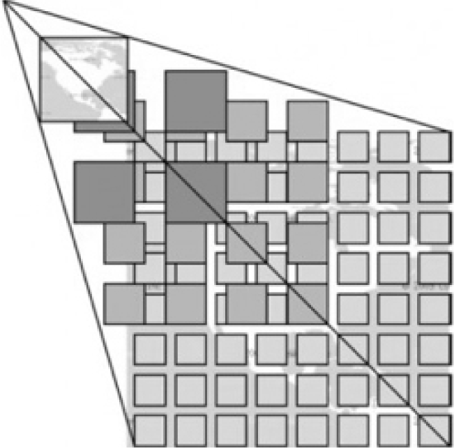
Hierarchical representation of Google Maps tiles, based on Mercator projection

2.3 Image Processing Techniques

The geographic satellite images of the target fields are processed using noise reduction, edge detection, colour reduction and median filtering methods to prepare the image for the determination of the boundaries and detection of obstacles.

2.3.1 Filtering and Noise Reduction

Median filtering is a nonlinear operation that is used to eliminate sharp singular marks, which are of no consequence due to their small size [8]. This filtering is preferred to others due to its potential to preserve edges, while suppressing noise.

2.3.2 Edge Detection Techniques

Edge detection is essential to find boundaries of the desired field and determine the specifications of obstacles like dimensions and location. It also helps to find the field's attributes such as length and position. Several edge detection techniques, including Prewitt, Sobel, Roberts and Canny, are utilized [25, 11]. After noise reduction, Prewitt, Sobel and Roberts had more acceptable results, based on the parameters used in this study and presented in Section 3.2. As shown in Figure 3, among these popular methods, Sobel - with no thinning - seems to perform the best in the detection and presentation of edges in an agricultural environment.

Figure 3.

Results of edge detection techniques, a) Sobel, b) Prewitt, c) Roberts and d) Canny

3. System Description

The proposed method mainly works on top-view satellite images, and is processed to detect the boundaries of the field and the obstacles, as described in [23]. Although different kinds of obstacles, such as stones and trees, may exist in an agricultural field, this study focuses on detecting trees to emphasize the validity of this method. The system contains four main stages, as shown in Figure 4, consisting of: 1) initialization, to locate and import the image; 2) field extraction, in which the target field is extracted; 3) obstacle detection, to detect, position and store obstacles; and 4) trajectory generation, which generates tracking trajectory points.

Figure 4.

Architecture of the proposed system containing four stages: initialization, field extraction, obstacle detection and tracking trajectory point generation

3.1 Field Extraction and Sectioning

Users entering any GPS coordinates of the agricultural field do the initialization of the system to target the desired field. This study takes advantage of thresholding methods, such as Otsu's method, to perform segmentation on the image for extraction of the target field and detection of obstacles [44]. The user determines the highest possible zoom level (A_z) that fits the field into the frame. The obtained image is converted to gray-scale for further processing by retaining the luminance, while eliminating the hue and saturation information. Conversion to gray-scale is obtained using the weighted sum of R, G, and B components of the imported colour image (0.2989×R+0.5870×G+0.1140×B) [41].

On the gray image, a median filtering with a 3-by-3-neighbourhood matrix is applied to reduce typical “salt and pepper” noises [8]. The target field is extracted from the imported image using segmentation techniques and sectioning [30, 6]. The proposed method also allows the user to tune the filtering parameters of the automated process interactively, which gives the user an opportunity to select the target field manually if needed. Then, a binary form of the image is constructed, as in Figure 5b. The detected regions (Ri) are numbered, based on the number of connected pixels (ni), as in Figure 5c. The centre of the image is mapped to the GPS coordinate of the field, and the largest region, which overlaps it, is considered to be the target field [42]. The imported image is cropped using the bounding box properties of the field to only show the desired field, as in Figure 5d and 5e.

Figure 5.

a) Original image, b) binary image, c) numbered regions, d) cropped image using bounding box and e) desired field

3.2 Obstacle Detection and Positioning

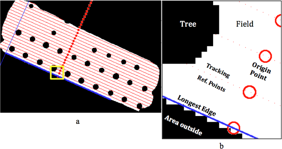
In this section, a method for detecting obstacles in an agricultural field is presented [23]. The undesired regions inside the field, which are too small to be deemed as obstacles, are removed using morphological image reconstruction by filling them [22, 16]. Top-view of trees in satellite images usually appear as a circle or ellipse, and are detected using Circular Hough Transform (CHT) [31]. The radius of trees has various ranges in different zoom levels. In this study, the CHT parameters are set to: object-polarity = ‘bright’, computation method = PhaseCode, sensitivity-factor = 0.9 and, finally, edge-gradient-threshold = 0.27.

Past experience shows that at Δ_z = 18, which this experiment is based on, trees have a radius range from 4–18 pixels, which changes in various zoom levels. The proposed method is designed to work with other zoom levels too. However, due to limited space in this article, the results will not be presented. Each detected circle to be accepted as a new tree entry is checked for duplicity. This is done by mapping the centre point of the object to a pixel in the image and searching the list to find duplicates. In the case of no duplication, the tree is stored with its centre pixel and radius (in pixels) to determine its diameter.

Captured satellite images are not set with GPS information. Therefore, we have proposed a positioning method to convert pixels to GPS coordinates. The system works on a geographic coordinate system, which is based on latitude and longitude. Starting with the earth's circumference at equator α = 40075017 metres for θ_e = 360°, the number of pixels in a tile p_t = 256 and p_z = z_t x 2Δz the number of pixels in zoom level (Δz) and the length of one degree of Longitude Per Pixel (LDPP) is determined by dividing θ_e over p_z. Additionally, by dividing α over p_z, the number of metres per pixel at the equator is calculated, which is 0.5971645 metres at Δz =18. While moving from the equator to the poles, the distance between longitudes gradually approaches zero, which means that the distance of one degree at the equator has its maximum value of 111319.49167 metres, and decreases as it approaches the poles, which was calculated in our previous study [23].

In addition, while moving towards the poles, the number of GPS points per pixel differs too. Therefore, to get an accurate position, another mapping is required. Multiplying longitude at each degree by the number of GPS points per pixel results in establishing an accurate position. The centre pixel of the image is mapped to the GPS point, which is provided by the user, as in Figure 6a. However, during field extraction, while cropping the image, the Original Centre Pixel (OCP) might be displaced, as in Figure 6b. In order to get an exact location, the offset needs to be calculated. From Figure 6b, the displacement of the centre pixel is obvious. To calculate this offset, Bounding-box's Start Point (BSP) and Bounding-box's End Point (BEP) (the dashed lines in Figure 6a) are used.

Figure 6.

Offset calculation of centre point

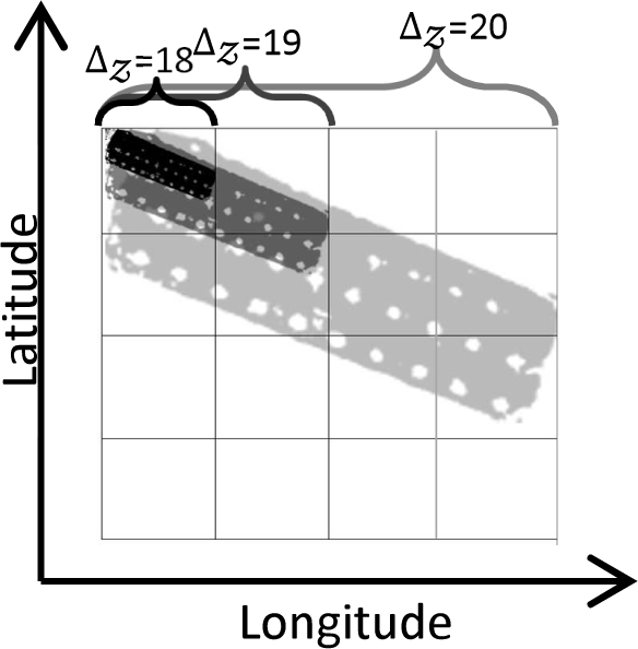
In this case, the values are (BSP (X_s, Y_s)) = (163.19, 173.11). The cropped centre pixel's new position and offset are calculated by subtracting OCP's coordinates from CCP's. The only GPS coordinates of the field provided by the user in latitude (r p_Lat) and longitude (r p_Long) are mapped to the centre pixel of the image, which all further positioning procedures depend on, hence, maintaining its exact location is essential. Having the offset calculated, the system can calculate each detected tree's exact coordinates in latitude and longitude pairs, using their centre pixel coordinate (tx_ti, ty_ti) using Eq. 1 and Eq. 2. After validation, the object is stored with its properties, such as index, position, pixel coordinates, radius, latitude and longitude, and is graphically annotated with a red circle [19, 14].

t_{L a t} = r p_{L a t} + ((C C P_{x} - t y_{t i}) \times (\cos \frac{r p_{L a t} \times π α}{180}) \times (\frac{θ_{e}}{P_{Z}}))

(1)

t_{L o n g} = r p_{L o n g} - ((C C P_{y} - t x_{t i}) \times (\frac{θ_{e}}{P_{Z}}))

(2)

3.3 Trajectory Points Generation and Positioning

The system provides a sequence of GPS trajectory points for agricultural vehicles to follow [35]. Having obtained all of the required data that are related to the field and obstacles therein, the sequence of tracking trajectory points in the form of a path is ready to be generated. The aim is merely to provide trajectories rather than path planning. To test the integrity of the proposed approach, the generated trajectory points are integrated into a simple path planning technique, which finds the longest edge and provides parallel lines according to that edge.

In the binary image, it is assumed that the pixels with value “one” (white colour) are referring to the main field, and the trajectory pints should be within these areas. The detected trees are re-plotted into the field using their centre point coordinate and radius in pixels as black regions with “zero” value after the field is filled with “one” values. This process results in a clearer, smoother and more precise image, containing both the field and the trees. Applying Standard Hough Transform (SHT) algorithm on the binary image results in finding the longest edge of the field. In the algorithm, the distance between the origin and the line (ρ_h) is set to 0.5 and the angle from the origin to the closest point (θ_h) is set to −90 ≥θ_h <89, respectively. During the search, each line's length is calculated using its first point coordinate (p1), last point coordinate (p2) and orientation angle θ_h (Eq. 3).

l_{l i n e} = \sqrt{{(p 2_{X} - p 1_{X})}^{2} + {(p 2_{Y} - p 1_{Y})}^{2}}

(3)

A line with maximum l_line value is stored as the longest edge (E D_max) along its θ_h. The slope of the longest line (m_EDmax) is calculated, as follows:

m_{E D_{m a x}} = \frac{p 2_{Y} - p 1_{Y}}{p 2_{X} - p 1_{X}}

(4)

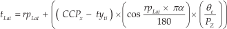
The E D_max is highlighted with a blue bold line, as shown in Figure 7a. Desired paths must be parallel to the E D_nmx with equal distance from each other. The distance between paths (d_m) in metres is converted to pixels using Eq. 5.

Figure 7.

Tracking trajectory point generation and representation in a) general, b) detail

d_{p i x} = \frac{256 \times d_{m} \times 2^{Δ_{z}}}{θ_{e}}

(5)

The desired paths are to be parallel to each other with constant d_pix, as entered by the user. Therefore, temporary points (red dots) are plotted as origin points to draw paths, as in Figure 7b. Any deviation of origin points will result in lines with unequal distance d_pix from each other. Midpoint (p_mid _x,y) of the ED_max is taken as the start point to draw the perpendicular lines.

p_{m i d}_{x, y} = ((\frac{p 1_{X} + p 2_{X}}{2}), (\frac{p 1_{y} + p 2_{y}}{2}))

(6)

O P_{x} = p_{m i d}_{x} + (Δ i n c \times (\sin m_{E D_{m a x}}))

(7)

O P_{y} = p_{m i d}_{y} + (Δ i n c \times (\cos m_{E D_{m a x}}))

(8)

The slope of the perpendicular line is m_pLine = atan (m_EDmax). Each origin point $(O P_{x, y})$ is placed one by one with a constant increment (Δ_inc) to generate points with equal distance from each other using Eq. 7 and Eq. 8. The system generates tracking trajectories using the longest edge, perpendicular line and origin points. A sequence of trajectory points in a straight line is generated by replacing m with m_pLine in linear equation y = mx + bEq. 9 and Eq. 10 Likewise, b (y-intercept) is replaced by $O P_{y}$ (y-coordinate of the origin point) and x is calculated by decrementing the origin point's x-coordinate from PL_x, which increments pixel by pixel to determine the offset.

P L_{x} = 1 t o i m a g e w i d t h

(9)

P L_{y} = (m_{E D_{m a x}} \times (P L_{x} - O P_{x})) + O P_{y}

(10)

These pixels represent the points in which tracks parallel to the longest edge should pass through. Any intersection between the trajectory points and detected obstacles in the field needs to be determined to avoid any collisions. The system maps each generated point's pixel coordinates (x, y) to the image and compares their value and, if it is overlapped with a pixel with a “zero” value, the point is discarded. This is due to the fact that either the generated point is placed on an obstacle or it is outside of the field's boundary, as both are presented with “zero” value. After passing all of the conditions, the trajectory points are plotted sequentially on the field as red dots in straight lines, as in Figure 7a.

Each trajectory point is converted from pixel to GPS coordinates to be used by a GPS tracking enabled agricultural vehicle [23]. As indicated, moving between the poles and equator results in different distances that each pixel can cover. Therefore, the exact length of a degree of longitude per pixel (LDPP) must be calculated [23]. Pixel-to-GPS conversion results are stored in a 2D-array (m × n) Table 1. Columns 1 to 4 contain information related to the first track, columns 5 to 8 contain information for the second track and so on. The first two are pixel coordinates (TP_xi, _yi ) and the next columns are GPS coordinates (TP_{Lat, Long}) of the trajectory point.

Table 1.

Format of the path's trajectory points in an array

Trajectory Points	X	Y	Lat.	Long.
Trajectory Points	5	6	7	8
23	63	12.391…	35.0755…	33.5308…
24	64	12.836…	35.0755…	33.5308…
25	65	13.281…	35.0755…	33.5308…
26	66	13.725…	35.0755…	33.5309…
27	67	14.170…	35.0755…	33.5309…
28	77	18.619…	35.0755…	33.5309…
29	78	19.064…	35.0755…	33.5309…
30	79	19.509…	35.0755…	33.5309…

4. Results

In order to illustrate the proposed method, a number of examples are presented. The system is developed and tested on MATLAB technical programming language (The MathWorks Inc., Natwick, MA) platform. A computer with a CPU of 2.8 GHz (Intel Core i7) and 8 GB of RAM running on a Mac OS X Yosemite (10.10.3) is used to run and test the system. All of the satellite images are obtained from Google Maps Image API with resolution of 640×640 pixels, as provided by Static Map API. The algorithm was tested on seven different fields with various shapes, sizes and number of obstacles to validate the system. The zoom level in all of the tests is set to 18 for comparison purposes. In addition, the radius range for the detection of trees regarding Δ_z = 18 is set to a minimum of $ℛ α_{m i n} = 4$ and a maximum of $ℛ α_{m a x} = 18$ in pixels. However, this is subject to change, depending on zoom level. After an extraction of each field, the original image is cropped to only contain the desired field, resulting in an image with different dimensions, as in Figure 8. Furthermore, the tree detection outputs of these fields are graphically presented with red circles in the images.

Figure 8.

Test fields after crop and obstacle detection

Details of the detection section for these seven fields are shown in Table 2. The columns from left to right are the total number of trees, the total number of tree detections, correct detections, incorrect detections, the accuracy of correct detections, the percentage of incorrect detection and the complexity of the field. Complexity is defined based on the number of obstacles, their shape, size, fields' dimensions and smoothness of edges. The distance between the desired paths are set to be d_m = 2 m in all of the fields for comparison purposes. Results of the path finding algorithm based on SHT are shown in Figure 9.

Table 2.

Data regarding the obstacle detection section

Field No	#. of Trees	# Det. Trees	Correct	Incorr.	Accu %	Error %	Compl.
1	2	1	1	0	50	0	1
2	2	2	2	0	100	0	1
3	1	1	1	0	100	0	1
4	3	3	3	0	100	0	2
5	26	26	26	0	100	0	2
6	17	19	16	3	94.117	17.647	3
7	194	131	130	1	67.010	0.5154	4
				Avg.	87.303	2.5946

Figure 9.

Results of generating sequence of trajectory points to form the desired path

5. Discussion

According to the experimental results, the system is capable of detecting obstacles with significant precision, while using the free Google Maps API, which provides a maximum 640×640 pixels image and forced us to use low zoom levels. The system's accuracy is correlated with zoom level, such that a higher zoom level results in more precise detections. Using Google Business API with an image of 2048 × 2048 pixels, the same experiment could be conducted with zoom level 20, resulting in an image with four times more clarity, as in Figure 10. In turn, this would increase the precision of detection. As previously presented in Table 2, the results indicate that, while the number of trees and complexity increases, the accuracy remains significant.

Figure 10.

Correlation between zoom and quality

Overall, the accuracy is above 80%, except for fields 1 and 7. The low accuracy in field 1 is due to the fact that one of the two trees in the field is covered by Google's watermark on the image, making the system unable to detect the tree. Additionally, in field 7, since many of the trees were together and formed, non-circular shapes resulted in the failure of detection. Table 2 shows that the average accuracy in the detection of trees and average error are more than 87% and less than 3% respectively, which represents a significant result.

Assuming that Google provides precise data, the proposed system proves to be successful in positioning. Coordinates of an obstacle detected and positioned by the proposed method is searched by Google Maps to validate its accuracy as an example. Figure 11 shows that the GPS coordinate points exactly to the centre of the detected tree.

Figure 11.

Coordinates of detected trees, validated with Google Maps (Lat: 35.218108, Long: 33.572233)

The proposed method is also accurate in calculating the detected obstacles' sizes, although they may appear in different sizes in the agricultural fields. As an example, the detected trees' diameter using the proposed method (Figure 12a) is 10.14 m (20.74 pixels in the image), from Google Maps is 10 m (Figure 12b) and its actual diameter, as recently measured, was 11.1 m (Figure 12c). A comparison between the detected trees' sizes calculated by the proposed method and Google Maps (14 cm difference) indicates a very low error rate in measuring obstacle sizes. However, the big difference between the actual size of the obstacle and the size provided by Google Maps indicates the insufficiency of Google Maps' accuracy in representing data.

Figure 12.

Measuring obstacle size using: a) the proposed method, b) Google Maps and c) actual size

The path planning strategy used in this study generates paths that are parallel to each other. A linear equation of the base line with different a y-intercept but constant increment is considered to guarantee the parallelism and straightness. Both tracks in the pixel and GPS coordinates are compared to validate the accuracy of conversion. From the line equations in the charts presented in Figure 13, it can be concluded that both lines in the pixel and GPS coordinates are straight lines and this is due to the fact that all of the exponents are not higher than one.

Figure 13.

Validation of straightness of tracking trajectory points both in the pixel and GPS coordinates

Furthermore, the coefficient of determination (R2) of the points with the value of 1 confirms the complete straightness of the both lines. The coefficient of determination of the trajectory points in both the pixel and GPS coordinates for all fields in this study are presented in Figure 14a. The results indicate that the points are less that 0.005% variation from the straight line, which shows that the conversion is significant.

Figure 14.

a): Coefficient determination of x,y and GPS coordinates, b) Standard deviation of the distance between tracking trajectory points in x, y and GPS coordinates.

In addition, it is necessary for these points to be equidistant from each other, which ensures that tracking devices would not lose or stray from the path. A low standard deviation result indicates the accuracy in generation and conversion of tracking trajectory points, as shown in Figure 14b. To investigate the computational times, the same experiments are performed with various distances (d_m = 2m, d_m = 4m, d_m = 6m) and the results are shown in Figure 15, which are in the range of 2.04s to 25.95s for d_m = 2m, 1.35s to 14.47s for d_m = 4m, and 1.15s to 10.69s for d_m = 6m. The results indicate that the computational time increases almost twofold by decreasing the distance between paths to half.

Figure 15.

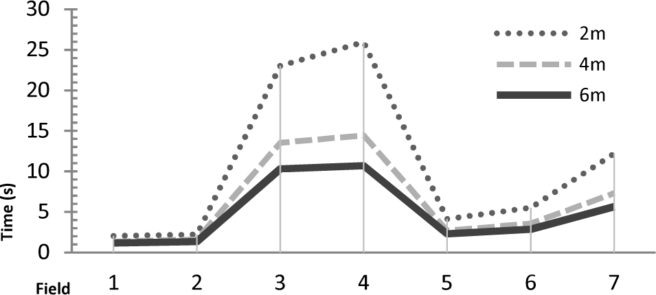
Computational time for 2, 4, and 6 m path distance in seven fields

Table 3 presents the processing time for all of the fields. From the table, it can be observed that the highest rates of processing time belong to fields 3 and 4, as they are almost twice the size of fields 1, 2, 5 and 6, which requires more trajectory points to cover the field.

Table 3.

Proceeding time for different fields with different shape, size and number of obstacles

Field	Track Distance
	2m				4m				6m
	Time	No. of Tracks	No. of segments	Total Kef. Points	Time	No. of Tracks	No. of segments	Total Ref. Points	Time	No. of Tracks	No. of segments	Total Ref. Points
1	2.04	28.00	35.00	2428.00	1.35	14.00	16.00	1213.00	1.15	10.00	13.00	808.00
2	2.22	64.00	72.00	2601.00	1.58	32 00	37.00	1325.00	1.34	22.00	26.00	877.00
3	23.04	106.00	128.00	37553.00	13.54	53 00	40.00	18776.00	10.31	36.00	29.00	12480.00
4	25.95	107.00	130.00	46027.00	14.47	54.00	69.00	23085.00	10.69	36.00	47.00	15436.00
S	4.13	20.00	62.00	5576.00	2.69	10.00	39.00	2684.00	2.29	7.00	15.00	1930.00
6	5.51	33.00	93.00	8422.00	3.55	1700	49.00	4226.00	2.86	11.00	35.00	2807.00
7	12.19	64.00	531.00	21140.00	7.29	32.00	286.00	9648.00	5.66	22.00	193.00	6438.00

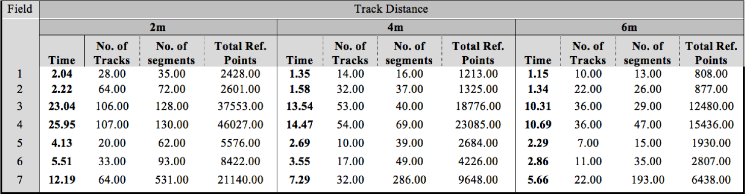
Although field number 7 is almost the same size as fields 3 and 4, the results from Table 2 indicate that the computational time and generated trajectory points are half as many. Table 1 shows that the system has detected one obstacle in field number 3, and three in field number 4, while, for field 7, there are 194 detected obstacles. Having more obstacles in the field results in less space for planting, which causes the system to eliminate those areas from the path. This results in a decrease in generation of tracking trajectory points and computational time.

6. Conclusion

In this study, a method for the generation and positioning of tracking GPS trajectory points for agricultural autonomous systems has been presented. The proposed method begins with a single GPS coordinate of an agricultural field, and detects obstacles automatically. The acquired global position and dimensions of detected obstacles can be used for agricultural vehicles to avoid any collisions. Low computational time in the range of 1.15 – 25.95 seconds, along with simplicity of use and accuracy in positioning and generating of tracking trajectory points, makes the proposed method feasible to be integrated into any path planning algorithm or method for automation of agricultural vehicles. The generated trajectory points are graphically represented in the image to be presented to the user. This method is tested with a simple path planning technique to validate the generation of trajectory points. According to the experimental results, the proposed method provides significant means to generate trajectory points and position obstacles. In the near future, this method can be extended to cover more types of obstacles, along with the development of other subsystems of agricultural automation such as interactive user interfacing for obstacle verification.

Footnotes

7. Acknowledgements

The authors wish to thank Anas MAHDI for his contribution to this study in the statistical analysis.

References

Bakhtiari

Navid

Mehri

Bochti

: Optimal Route Planning of Agricultural Field Operations Using Ant Colony Optimization. Agricultural Engineering International: CIGR Journal. 2011; 13, No.4.

Anita

Liang

Gauri

Salokhe

Margherita

Sini

Johannes

Keizer

: Towards an Infrastructure for Semantic Applications: Methodologies for Semantic Integration of Heterogeneous Resources. Cataloging & Classification Quarterly. 2006:43:161–189.

Anuj

Mohan

Constantine

Papageorgiou

Tomaso

Poggio

: Example-Based Object Detection in Images by Components. IEEE Transactions on Pattern Analysis And Machine Intelligence.;2001:23(4): 349–361.DOI: 10.1109/34.917571.

Antonio

Sgorbissa

Renato

Zaccaria

: Integrated Obstacle Avoidance and Path Following Through a Feedback Control Law. J Intell Robot Syst. 2013;72:409–428. DOI 10.1007/s10846-012-9806-2.

Bin

J-Stilwell

Daniel

J-Kurdila

Andrew

: Fast Path Re-planning Based on Fast Marching and Level Sets. J Intell Robot Syst.2013;71:303–317.DOI: 10.1007/s10846-012-9794-2.

Chen

Tao-Ruan

Ian

J-P

: Automatic Reconstruction Of 3D Environment Using Real Terrain Data and Satellite Images. Intelligent Automation and Soft Computing.2012;18(1):49–63. DOI: 10.1080/10798587.2012.10643226.

Dragos

Ion

Mihai

: Bridging the Semantic Gap for Satellite Image Annotation and Automatic Mapping Applications. IEEE Journal of Selected Topics in Applied Earth Observations and Remote Sensing.2011;4(1): 193–204. DOI: 10.1109/JSTARS. 2010.2081349.

Maheswari

Radha

: Noise Removal in Compound Image Using Median Filter. IJCSE International Journal on Computer Science and Engineering. 2010; 2(4):1359–1362.

Erik

Noé

Ortega-S

Daniel

Pérez-Cisneros

Marco

: Circle Detection by Harmony Search Optimization. J Intell Robot Syst.2012;66:359–376. DOI 10.1007/s10846-011-9611-3.

10.

Fabre

Philippe

Michel

Lionel

: Framework Path Planning for Field Coverage with Minimum Overlapping, international Conference on Emerging Technologies and Factory Automation, Proceedings. IEEE;2001. P. 691–694.

11.

Shrivakshan

Chandrasekar

: A Comparison of Various Edge Detection Techniques Used in Image Processing. IJCSI International Journal of Computer Science Issues.2012;9(5–1), ISSN (Online): 1694-0814.

12.

Google: Google Map API. Available from: https://developers.google.com/maps/documentation. Accessed on 23 Dec 2013.

13.

Guoyu

Peng

Junfei

: Path Planning Algorithm Based on Sub-Region for Agricultural Robot. 2nd International Asia Conference on Informatics in Control, Automation and Robotics; 6–7 March 2010; Wuhan; 2012. P. 197–200.

14.

Hei-Chia

Tian-Hsiang

Chia-Tzung

: Automatic Summarization Based on Automatically Induced Ontology. Intelligent Automation and Soft Computing. 2011;17(4):447–463. DOI. 10.1080/10798587.2011.10643160.

15.

Hameed

Bochtis

Sørensen

Nøremark

: Automated Generation of Guidance Lines for Operational Field Planning. Bio Systems Engineering.2010;107;294–306. DOI: 10.1016/j.biosystemseng. 2010.09.001.

16.

Jiann-Jone

Chun-Rong

W-Eric

Jun-Lin

De-Hui

: Object Segmentation of Database Images by Dual Multiscale Morphological Reconstructions and Retrieval Applications. IEEE Transactions on Image Processing.2012;21(2):828–43. DOI: 10.1109/TIP.2011.2166558.

17.

Jacek

Tomas

Carine

Joel

: SAWSDL: Semantic Annotations for WSDL and XML Schema. Internet Computing, IEEE.2007;11(6):60–67. DOI: 10.1109/MIC.2007.134.

18.

Kevin

Antonio

Daniel

William

: Object Detection and Localization using Local And Global Features. Toward Category-Level Object Recognition Lecture Notes in Computer Science Volume 4170; 2006. P. 382–400. DOI: 10.1007/11957959_20.

19.

Kuhanandha

Michael

N-H

: Ontology Tools for Semantic Reconciliation in Distributed Heterogeneous Information Environment. Intelligent Automation and Soft Computing.2000. p. 1–8.

20.

Kise

Noguchi

Ishii

: Laser Scanner-Based Obstacle Detection System for Autonomous Tractor-Movement and Shape Detection Targeting at Agricultural Vehicle. Journal of the Japanese Society of Agricultural Machinery.2005;66(2): 97–104.

21.

Kosmas

Stephan

Carsten

Nikos

Stamatia

Vassilis

Siegfried

Yannis

Yiannis

Steffen

: Knowledge Representation and Semantic Annotation of Multimedia Content. IEE Proc.-Vis. Image Signal Process.2006;153(3):255–262. DOI: 10.1049/ip-vis:20050059.

22.

Luc

Vincent

: Morphological Grayscale Reconstruction in Image Analysis: Applications and Efficient Algorithms. IEEE Transactions on Image Processing, technical report 91-16, Harvard Robotics Laboratory, November 1991, IEEE Transactions on Image Processing, 1993. P. 176–201.

23.

Mehmet

Moein

: Textual Annotation, Detection and Positioning of Obstacles in Agricultural Fields Using Satellite Images. ICSCCW-2013 Seventh International Conference on Soft Computing, Computing with Words and Perceptions in System Analysis, Decision and Control. Izmir, Turkey September 2–3, 2013.

24.

Mehmet

Ehsan

Hasan

: Double Look-ahead Reference Point Control for Autonomous Agricultural Vehicles. Biosystems Engineering, 2012; 113(2):173–186. DOI: 10.1016/j.biosystemseng. 2012.07.005.

25.

Mamta

Parvinder

: Performance Evaluation of Edge Detection Techniques for Images in Spatial Domain. International Journal of Computer Theory and Engineering.2009;1(5):614–621. DOI: 10.7763/IJCTE.2009.V1.100.

26.

Milan

Bojicb

Djordje

: Short- and Long-term Dynamic Accuracies Determination of Satellite-based Positioning Devices Using a Specially Designed Testing Facility. Computers and Electronics in Agriculture. 2011; 76(2):297–305. DOI: 10.1016/j.compag.2011.02.008.

27.

Mangal

Ian

: A Probabilistically Robust Path Planning Algorithm for UAVs Using Rapidly-exploring Random Trees. J Intell Robot Syst. 2013;71:231–253. DOI: 10.1007/s10846-012-9776-4.

28.

Marie

Henri

Mihai

: Semantic Annotation of Satellite Images Using Latent Dirichlet Allocation, IEEE Geoscience and Remote Sensing Letters, 31 July 2009. TELECOM Telecom ParisTech, Paris. 2010. P 28–32.

29.

Nørremarka

Griepentrogb

Nielsenb

Søgaardc

: The Development and Assessment of the Accuracy of an Autonomous GPS-based System for Intra-row Mechanical Weed Control in Row Crops. IAgrE. Published by Elsevier Ltd. 2008; 101(4):396–410. DOI: 10.1016/j.biosystemseng 2008.09.007.

30.

Muhammad

Abdul

Adil

M-S

: Image Segmentation Using Multilevel Graph Cuts and Graph Development Using Fuzzy Rule-based System. IET Image Process., 2013;7(3):201–211. DOI: 10.1049/jet-ipr.2012.0082.

31.

Marcin

Ignacy

: Circular Object Detection Using a Modified Hough Transform. Int. J. Appl. Math. Comput. Sci. 2008; 18(1):85–91. DOI: 10.2478/v10006-008-0008-9.

32.

Michel

Philippe

Helene

Lionel

: Path Planning for Complete Coverage with Agricultural Machines. Field and Service Robotics, Springer-Verlag Berlin Heidelberg 200. 2006. P. 549–558. DOI: 10.1007/10991459_53.

33.

Robert

David

M-B

: The Use of GPS for Vehicle Stability Control Systems. IEEE Transactions On Industrial Electronics. 05 April 2004. p. 270–277.

34.

Rahul

Kevin

: Multi-Level Planning for Semi-autonomous Vehicles in Traffic Scenarios Based on Separation Maximization. J Intell Robot Syst. 2013; 72:559–590, DOI: 10.1007/s10846-013-9817-7.

35.

Roland

Benoit

Christophe

Philippe

: High Accuracy Path Tracking for Vehicles in Presence of Sliding: Application to Farm Vehicle Automatic Guidance for Agricultural Tasks. Autonomous Robots. 2006;21(1):79–97. DOI: 10.1007/s10514-006-7806-4.

36.

Roland

Benoit

Christophe

Philippe

: Adaptive and Predictive Path Tracking Control for Off-road Mobile Robots. European Journal of Control. 2007;13(4):419–439. DOI: 10.3166/ejc.13.419-439.

37.

Simon

Yang

C-L

: A Neural Network Approach to Complete Coverage Path Planning. IEEE Transaction on Systems Man and Cybernetics Part B: Cybernetics. 2004. p. 718–724

38.

Thomas

Daniel

Hermann

: Discriminative Training for Object Recognition Using Image Patches. IEEE Computer Society Conference on Computer Vision and Pattern Recognition (CVPR'05), Feb 2005.

39.

Oksanen

Visala

: Path Planning Algorithms for Agricultural Machines. Agricultural Engineering International: The CIGR Ejournal. Manuscript ATOE 07 009. IX. Feb 2007.

40.

Victor

Luisa

Yolanda

Justo

: Planning for Agricultural Forage Harvesters and Trucks: Model, Heuristics, and Case Study. Networks & Spatial Economics - NETW SPAT ECON. 2010;10(3): 321–343. DOI: 10.1007/s11067-009-9120-0.

41.

Wain

Nyein

: On the Automatic Detection System of Stop Line Violation for Myanmar Vehicles (Car). International Journal of Computer & Communication Engineering Research (IJCCER). 2013;1(4), e-ISSN: 2321-4198 p-ISSN: 2321-418X.

42.

Yu-Wing

Jiaya

Chi-Keung

: Soft Color Segmentation and Its Applications. 29 September 2007 IEEE Transactions on Pattern Analysis and Machine Intelligence. 2007. p. 1520–1537.

43.

Zhang

Qiu

: A Dynamic Path Search Algorithm for Tractor Automatic Navigation. Transactions of the ASAE. 2004; 47(2). DOI: 10.13031/2013.16027.

44.

Nobuyuki

: A Threshold Selection Method from Gray-Level Histograms. IEEE Transactions on Systems, Man, and Cybernetics. 1979 p. 62–66.

Satellite Images-Based Obstacle Recognition and Trajectory Generation for Agricultural Vehicles

Abstract

Keywords

1. Introduction

2. Preliminaries

2.1 Source of Satellite Images

2.2 Positioning System

2.3 Image Processing Techniques

2.3.1 Filtering and Noise Reduction

2.3.2 Edge Detection Techniques

3. System Description

3.1 Field Extraction and Sectioning

3.2 Obstacle Detection and Positioning

3.3 Trajectory Points Generation and Positioning

4. Results

5. Discussion

6. Conclusion

Footnotes

7. Acknowledgements

References