Sage Journals: Discover world-class research

Abstract

Rough-terrain traversability is one of the most valuable characteristics of walking robots. Even despite their slower speeds and more complex control algorithms, walking robots have far wider usability than wheeled or tracked robots. However, efficient movement over irregular surfaces can only be achieved by eliminating all possible difficulties, which in many cases are caused by a high number of degrees of freedom, feet slippage, frictions and inertias between different robot parts or even badly developed inverse kinematics (IK). In this paper we address the hexapod robot-foot deviation problem. We compare the foot-positioning accuracy of unconfigured inverse kinematics and Multilayer Perceptron-based (MLP) methods via theory, computer modelling and experiments on a physical robot. Using MLP-based methods, we were able to significantly decrease deviations while reaching desired positions with the hexapod's foot. Furthermore, this method is able to compensate for deviations of the robot arising from any possible reason.

Keywords

Hexapod Robot Inverse Kinematics Neural Network Foot Error Error Compensation

1. Introduction

Walking robots show much greater ability to traverse terrain than wheeled or tracked robots. Although wheeled robots have higher speed and simple control methods, walking robots would be preferred for difficult terrain missions such as planetary exploration, underground operations or catastrophic environments.

However, walking robots are still far from being exhaustively researched and produced. Problems like high energy consumption, difficult gait selection, complex control and feet placement arise when moving over rough terrain. Each problem must be considered and eliminated before using robots in any real-life situation. In this paper, we propose MLP-based methods for reducing deviations of a hexapod robot's leg that appear when using a geometric inverse-kinematics method.

Having precise inverse-kinematics calculations are very important, because trajectory planning requires inverse-kinematics solutions; they are also necessary when executing delicate tasks. Relatively small deviations when calculating joint-space coordinates often cause unacceptable deviations in Cartesian space coordinates.

There are three traditional methods used to solve inverse kinematics [1]: geometric [2, 3], algebraic [4, 5, 6, 7] and iterative [8]. These methods can become complex and time consuming when used in complex systems. In addition, these methods only give a solution for a fixed geometrical configuration of the kinematic chain; if the kinematics change, for example, a robot's leg is damaged, it is necessary to find a new inverse-kinematics solution.

Many different intelligent methods (based on neural networks, fuzzy logic, reinforcement learning, etc.) were proposed to solve the inverse-kinematics problem of different robotic systems [9, 10, 11, 12]. These methods proved capable of overcoming the problems of traditional methods and they also provide a good basis for adaptive kinematic solutions that are not constrained by robot kinematics.

Many reasons remain as to why deviations of feet coordinates or leg trajectories appear. When the number of manipulator degrees of freedom increases, and structural flexibility is included, analytical modelling becomes almost impossible [13]. Even a simple, real-world rigid structure displays errors when compared to a modelled structure. Furthermore, mechanical wear and structural flexibility adds more error to the system. After some usage, the system requires recalibration to perform as expected. Analytical methods of solving inverse-kinematics problems become insufficient.

Another possible source of the problem is feet slippage [14]. Moosavian et. al. have developed a dynamic model for a hexapod robot which consists of only a narrow pack of equations. This model includes feet interaction with the ground and a force distribution model to find the required friction forces. Even though the experimental results showed minimum slippage, it is still obvious that the deviation has not been avoided fully.

It has been proposed by several scientists [15, 16] that leg trajectory errors might occur due to a poorly developed inverse-kinematics model. Robots with legs are very complex systems consisting of a large number of actuators, joints and other elements. Both the complexity of the kinematic model and control over it increase with the presence of more parts. Therefore, dynamic models and control algorithms must be carefully organized. Accurate control of all actuator speeds is also very important. As the speed increases, completing various operations and the useful workspace of the leg or manipulator reduces the effect described in [17]. In addition to actuator speeds, sometimes joint frictions and inertias, as well as some external disturbances, are not known [18]. Having to take all of these conditions into account makes eliminating feet-positioning deviations a very difficult task.

2. Hexapod robot description and leg kinematics

For our experiments, a typical hexapod robot with a total of 18 degrees of freedom (DoF) was used. Each leg has three Dynamixel AX-12+ servomotors (giving each leg 3 DoF). AX-12+ actuators support a 10 V input voltage and a 900 mA maximum current. The working angle is 300° with a 0.35° resolution. The robot used is relatively small: body length L₁ = 160 mm and width L₂ = 90 mm. Leg dimensions are as follows: l₁ = 80 mm, l₂ = 106 mm and l₃ = 68 mm (see Figure 2). The total weight of the robot is around 1.5 kg, consisting mostly of 18 actuators, each of which weighs 55 g.

Figure 1.

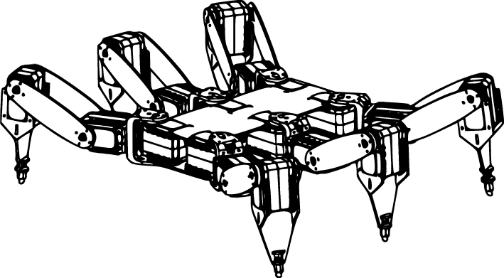
Hexapod robot CAD model

Figure 2.

Robot leg projections into xy (a) and xz (b) planes

The analysis of a robot's whole kinematic model can be simplified by taking each leg as an individual system [16]. The leg design is very similar to a bug's leg, as explained in detail in paper [19]. As each hexapod robot's leg has 3 DoF, inverse kinematics can be easily calculated using a simple geometrical approach. Two leg projections are needed in order to derive servomotor angles, projection into xy (Figure 2 (a)) and xz (Figure 2 (b)) planes.

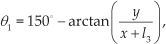
This method requires five equations (1 –5) to calculate three actuator angles from three given spatial-foot coordinates.

θ_{1} {= 150}^{\circ} - \arctan (\frac{y}{x + l_{3}}),

(1)

θ_{2} {= 150}^{\circ} - \arccos (\frac{l_{1}^{2} - l_{2}^{2} + B^{2}}{2 l_{1} B}) + \arcsin (\frac{z}{B}),

(2)

θ_{3} = 150 ° - (90 ° - \arccos (\frac{l_{1}^{2} + l_{2}^{2} - B^{2}}{2 l_{1} l_{2}})),

(3)

B = \sqrt{l_{4}^{2} + z^{2}},

(4)

l_{4} = \sqrt{x^{2} + y^{2}} .

(5)

Where:

θ₁ - angle of the coxa servomotor,

θ₂ - angle of the femur servomotor,

θ₃ - angle of the tibia servomotor,

B - subsidiary imaginary line, connecting the beginning of the femur and the end of the tibia,

l₁ - length of the femur,

l₂ - length of the tibia,

l₃ - distance between the coxa and femur axes,

l₄ - length of B projection to xy plane.

3. Experiment set-up and initial experiments

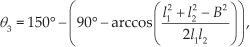
In order to test the foot's positioning accuracy and evaluate positioning errors, only one leg of the robot was used in the experiments. The leg was connected to the computer via USB to an UART converter (Figure 3). As no feedback from the servomotors was used, only the Tx line was used to transmit commands. Throughout the experiments, the servomotor's speed was always set to 5 RPM; this ensured less jerky leg motions. The foot's coordinates were measured in two-dimensional space, in xy plane. In order to measure the foot's real coordinates, they were marked on a piece of millimetre paper (Figure 4) after sending a command to position the leg at a certain set of coordinates. In this way, we were able to measure the real coordinates at which the foot was positioned. By comparing the desired coordinates that were sent to the leg with the real measured coordinates, we were able to evaluate the foot's coordinate deviations and positioning errors.

Figure 3.

Diagram showing the robot leg's connection to a PC

Figure 4.

Experiment set-up, showing the initial foot position (0, 0) and positive and negative foot-movement directions along the x and y axes (+X, -X, +Y, -Y)

3.1 Initial foot-position accuracy experiments

In order to measure foot-position deviation, the following experiment was carried out. The robot's foot was positioned at 55 different positions in its workspace; 27 of these positions were along the x and y axes, while one of the coordinates remained equal to zero. Another 28 positions were along the diagonal axes, when both x and y coordinates changed (Figure 5 blue dots). The leg was positioned on each point five times. The measurement results are shown in Figure 5 as green dots. This gave general information on what the positioning deviations are in different workspace areas. It can be noticed that deviations are very small along the positive x axis (when y = 0), and along the diagonal axes in the positive x axis (Ist and IVth quadrants). Deviations increase a little along the negative x axis (when y = 0) and along the y axis in both positive and negative directions. Deviations are the largest in diagonal directions on the negative x axis' side (IInd and IIIrd quadrants). The most important point, here, is that as the required position coordinates increase, deviations also increase, but only on the negative x axis' side and only slightly on both y axes' sides. This suggests that there may be problems for the leg moving in a negative direction, which may be caused by the fact that this direction is moving towards the robot's body and the position is close to the leg's mechanical limits. Other problems may arise from the coxa's servo because it is responsible for the leg's motion along the y axis. An explanation for this may be that the PID controller configuration is wrong for the said servo or even for all three servos. If this is the case, each servo controller must be configured, which may be time consuming and tedious work. Furthermore, PID controllers work only under certain constant conditions and if these conditions change for any reason, the PID controller must be reconfigured, which increases the problem still further. This also shows that even a simple geometric inverse-kinematics solution for 3 DoF leg may have problems. In this paper, we focus only on eliminating deviations that may appear for any known or unknown reasons with a neural network. As the hexapod robot is intended to be used in highly irregular terrain, it is essential to use adaptive methods for foot-trajectory correction. Nevertheless, the mentioned problems that may influence these deviations are interesting topics for future work (see Section 6).

Figure 5.

Initial experiment results that show foot-positioning deviations in different leg's workspace areas

4. Multilayer Perceptron-based method

Multilayer Perceptron (MLP) was chosen in order to compensate for errors that occur while positioning the robot's foot. To successfully solve this problem, a suitable MLP model was constructed (as described in Section 4.2). Training and testing data were gathered from a physical robot (as described in Section 4.2). Additional features were extracted by transforming points in Cartesian coordinate space to polar coordinate space, and data were normalized, as described in Section 4.1. To verify the results, experiments were carried out using a physical robot model.

4.1 Data preparation

The desired foot-position coordinates (x,y) were used as input parameters of the MLP-based method. MLP output-parameters are calculated joint angles (θ₁,θ₂,θ₃) needed to reach this desired position (x,y). After commanding the robot's leg to reach a desired position, the foot's coordinates were measured as described in Section 3. To increase accuracy, additional features were constructed by transforming the desired position in Cartesian coordinate space (x,y) to polar coordinate space (r,φ). Polar coordinates are interpreted in a more natural way, as they represent the distance and angle of the desired position. Experiments showed that when using both Cartesian and polar coordinates as input parameters, MSE converges to 0.1, Cartesian to only 0.57 MSE and polar to only 1.42 MSE. The learning speed also improved significantly, meaning that fewer iterations are needed for the MLP to converge. Constructing additional features from existing data is a technique widely used in neural networks, e.g., using polynomial inputs. A dataset of four input vectors X = (x,y,r,φ) and three output vectors Y =(θ₁,θ₂,θ₃) was constructed. Finally, each input and output vector was normalized by standard normalization (Equation 6, where x denotes the vector being normalized, μ is the mean, σ is the standard deviation of the dataset and z is the normalized vector).

z = \frac{x - μ}{σ} .

(6)

4.2 Constructing the MLP

It is a well-known fact that an MLP with one hidden layer exists that is capable of estimating an arbitrary nonlinear function to any desired level of accuracy [20, 21]. This is valid for acquiring training data. Our experiment also confirmed this, as the training error was close to the mechanical accuracy of the robot.

An MLP was constructed with four inputs, one hidden layer with six nodes and three outputs (Figure 6) (as described in Section 4.1). The number of nodes in the hidden layer was determined by an experiment (Figure 8). The mean squared error was measured on training data, running the MLP 100 times with different random weights at the intervals [-0.2; 0.2]. The standard deviations of 100 results were also measured to evaluate the stability of the MLP's configuration.

Figure 6.

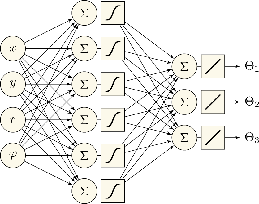
MLP architecture: four inputs {x,y,r,φ) representing coordinates in Cartesian and polar coordinate space; three outputs (θ₁,θ₂,θ₃) representing three joint angles; six nodes in a hidden layer with sigmoid activation functions and three output nodes with linear activation functions are being used

Figure 7.

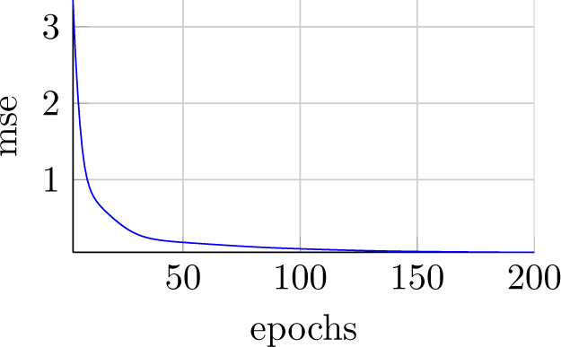
MLP's training error

Figure 8.

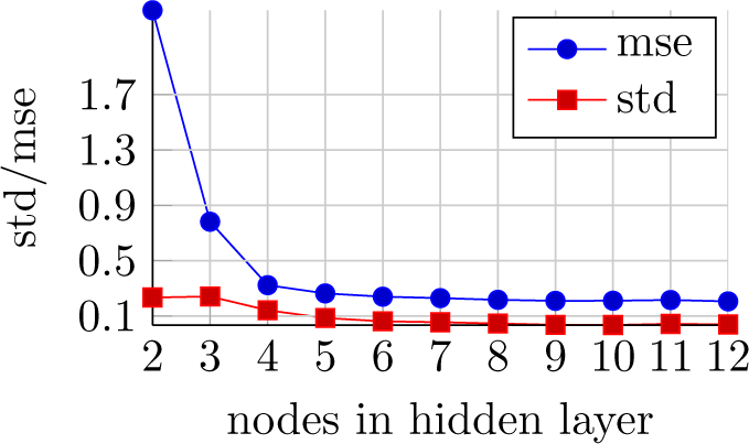
Nodes count in a hidden MLP layer's impact on performance

The MLP was trained for 200 epochs (Figure 7), with a learning-rate (η) value of 0.2 and a momentum factor (α) of 0.4. These values were chosen by means of experiment and were not critical. The MLP was able to continuously produce similar results (Figure 8). By increasing the epochs' count, smaller error rates could be achieved for the training data, but the testing data were barely affected. It is also significant that the robot's hardware only accepts integer numbers as joint-position parameters; therefore, a further increase of accuracy in training data was not needed.

Using sigmoid, stepper, soft-max or similar activation functions in the output layer can sometimes be beneficial (e.g., to force the output values to normalize between zero and one), but the linear activation function was preferred in this experiment because a continuous output was needed and data normalization was done separately. A sigmoid activation function was used in a hidden layer of the MLP.

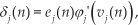
The MLP was trained using the delta rule (Equations 7 and 8).

Δ w_{j i} (n) = α Δ w_{j i} (n - 1) + η δ_{j} (n))_{i} (n),

(7)

δ_{j} (n) = e_{j} (n) φ_{j}' (v_{j} (n)),

(8)

φ_{j} (v_{j} (n)) = \frac{1}{1 + \exp (- v_{j} (n))} .

(9)

5. Experiment results

After training, the MLP's testing was performed on a physical robot. Deviations (D) were measured as the distance (in mm) from the desired position (coord_desired) to the actual position (coord_actual): D= | coord_desired-coor d_actual |, where coord is either the x or y coordinate. For this experiment, two positioning squares were used: one in the positive quadrant (Ist) and one in the negative quadrant IIIrd) (see Figure 9). The square in Ist quadrant represents the most accurate foot positions, as results of previous experiments showed minimum foot errors in this zone, while the square in IIIrd quadrant represents the least accurate zone (see Figure 5). Only these two quadrants were investigated, because they represent data inaccuracies in other two quadrants; that is, quadrants I and IV are symmetric and quadrants II and III are symmetric in accordance with positioning accuracy. Therefore, using all four quadrants would produce redundant information. For testing IK, the robot was only programmed to position its foot at certain positions, that are presented as green points (shown in Figure 9). After training, the MLP robot was reprogrammed to position its foot at different locations, presented as red points (Figure 9).

Figure 9.

Coordinate system with test points for the analytical method (green points) and for the MLP (red points)

Figure 10.

Experimental results in the positive xy plane, Ist quadrant, using the geometric IK method. Blue dots represent the desired positions and green dots represent the real measured positions.

Figure 11.

Experimental results in the positive xy plane, Ist quadrant, using the MLP method. Blue dots represent the desired positions and green dots represent the real measured positions.

Testing results can be seen in Figures 10 to 13. Experimental results with IK (Expr. 1) are shown in Figures 10 and 12. It is clear that the foot's position deviates more from the desired position in negative space (IIIrd quadrant) than in positive space; this also proves our earlier assumption. In positive space, the average deviation is 2.09 mm for the x coordinate and 1.53 mm for the y coordinate, and errors are ±0.21 and ±0.29 mm, respectively (Table 1). In negative space, deviations are noticeably bigger. The average deviations are 12.4 mm for the x axis and 19.6 mm for the y axis, with the errors ±0.17 and ±0.41 mm. respectively (Table 1).

Table 1.

Experimental results' comparison

	Expr. 1		Expr. 2
	x, mm	y, mm	x, mm	y, mm
Analytical method deviations	2.09	1.53	12.4	19.6
Error	±0.21	±0.29	±0.17	±0.41
MLP deviations	1.13	1.34	0.919	1.28
Error	±0.16	±0.24	±0.15	±0.28

Figure 12.

Experimental results in the negative xy plane, IIIst quadrant, using the geometric IK method. Blue dots represent the desired positions and green dots represent the real measured positions.

Figure 13.

Experimental results in the negative xy plane, IIIst quadrant, using the MLP method. Blue dots represent the desired positions and green dots represent the real measured positions.

Figures 11 and 13 show experimental results with a trained neural network (Expr. 2). It is obvious that deviations decrease dramatically, with average deviations of 1.13 mm for the x axis and 1.34 mm for the y axis in positive space, and 0.919 mm for the x axis and 1.28 mm for the y axis in negative space. Average errors are ±0.16, ±0.24 mm in positive and ±0.15, ±0.28 mm in negative spaces, respectively. As deviations with a trained MLP remain relatively the same in positive and negative spaces, it is safe to say that the MLP has learned to compensate for unnecessary foot deviations. Measurement errors also decreased, although by a very small margin and they remained almost the same, allowing us to say that the experimental results are reliable.

Table 1 shows the MLP-based inverse-kinematics' deviations in comparison with the analytical method.

6. Conclusions and future work

Theoretical calculations and experiments using a physical hexapod robot showed that using a simple Multilayer Perceptron can be beneficial for calculating inverse kinematics, as analytical methods cannot adapt to the inaccuracies and structural flexibility of robot mechanics. Practical experiments showed that, on average, the robot's foot deviates by 2.09 ± 0.21 mm on the x axis, and 1.53 ± 0.29 mm on y the axis, on the positive xy plane. In addition, the foot deviates by an average of 12.4 ± 0.17 mm on the x axis, and 19.6 ± 0.41 mm on the y axis, on the negative xy plane. Such deviations appear due to mechanical inaccuracies in using the analytical IK method for calculating servomotor angles. After calculating servomotor angles using a neural network, these deviations reduce to: x = 1.13 ± 0.16 mm, y = 1.34 ± 0.24 mm in the positive xy plane, and x=0.919 ± 0.15 mm, y = 1.28 ± 0.28 mm in the negative xy plane.

The MLP's configuration was not critical, and showed similar results when enough nodes in the hidden layer were used (Figure 8). On the other hand, data normalization was essential, and showed best results when each data vector was normalized by standard normalization.

One of the problems with our suggested method is that it makes it difficult to generate an automated robot's foot-position feedback. Therefore, this method cannot be used for autonomous robots without external supervision and future work would include development of the system with external foot-position supervision to be used as feedback for the MLP. Furthermore, future work will be carried out to determine the cause of the mentioned foot deviations by first changing the PID controller's configuration for each servo and determining how different controller configurations influence foot-positioning accuracy. If this method reduced foot deviations then we will also compare it to our suggested method in this paper.

Footnotes

7. Acknowledgements

This research was funded by grant MIP 057/2013 from the Research Council of Lithuania.

References

Köker

Öz

Cakar

Ekiz

A study of neural network based inverse kinematics solution for a three-joint robot. Robotics and Autonomous Systems. 2004; 49(3): 227–234. DOI:10.1016/j.robot. 2004.09.010

Featherstone

Position and velocity transformations between robot end effector coordinates and joint angles. The International Journal of Robotics Research. 1983; 2(2): 35–45. DOI: 10.1177/027836498300200203

Lee

C.S.G.

Robot arm kinematics, dynamics, and control. Computer. 1982; 15(12): 62–80. DOI: 10.1109/MC.1982.1653917

Duffy

Roth

Analysis of mechanisms and robot manipulators. Journal of Applied Mechanics. vol. 48, issue 1; 1980. p. 214. DOI: 10.1115/1.3157585

K.S.

Gonzalez

R.C.

Lee

C.S.G.

Robotics: control, sensing, vision, and intelligence. Industrial Robot: An International Journal. 1999. p. 580. DOI: 10.1108/ir.1999.04926bae.002

Manocha

Canny

J.F.

Efficient inverse kinematics for general 6r manipulators. Robotics and Automation, IEEE Transactions. 1994; 10(5): 648–657. DOI: 10.1109/70.326569

Paul

R.P.

Shimano

Kinematic control equations for simple manipulators. In: IEEE Conference on Decision and Control, 10–12 January 1979; San Diego, CA, USA: IEEE; 1978. pp. 1398–1406

Korein

J.U.

Badler

N.I.

Techniques for generating the goal-directed motion of articulated structures. In: IEEE Computer Graphics and Applications, Issue No.09 November 1982; Pennsylvania, USA: IEEE; 1982. pp. 71–81

Morris

A. S.

Mansor

Finding the inverse kinematics of manipulator arm using artificial neural network with lookup table. Robotica. 1997; 15(6): 617–625. DOI: 10.1017/S026357479700074X

10.

Alavandar

Nigam

M. J.

Neuro-fuzzy based approach for inverse kinematics solution of industrial robot manipulators. Int. J. of Computers, Communications and Control. 2008; 3(3): 224–234.

11.

Shah

Jolly A

Rattan

S. S.

Nakra

B. C.

Kinematic analysis of 3-DOF planer robot using artificial neural network. IAES International Journal of Robotics and Automation (IJRA). 2012; 1(3): 145–151. DOI: 10.11591/ijra.vli3.511

12.

Nanda

S. K.

Panda

Subudhi

P. R. S.

Das

R. K.

A novel application of artificial neural network for the solution of inverse kinematics controls of robotic manipulators. International Journal of Intelligent Systems and Applications (IJISA). 2012; 4(9): 81–91.

13.

Daya

Khawandi

Akoum

Applying neural network architecture for inverse kinematics problem in robotics. Journal of Software Engineering and Applications. 2010; 3(3): 230–239. DOI: 10.4236/jsea.2010.33028

14.

Moosavian

Ali

Dabiri

Dynamics and planning for stable motion of a hexapod robot. International Conference on Advanced Intelligent Mechatronics. 2010: 818–823. DOI: 10.1109/AIM.2010.5695819

15.

Roy

S. S.

Dilip

K. P.

Kinematics, dynamics and power consumption analyses for turning motion of a six-legged robot. Journal of Intelligent and Robotic Systems 74. 2014: 663–688. DOI: 10.1007/s10846-013-9850-6

16.

Duan

Chen

Liu

Tripod gaits planning and kinematics analysis of a hexapod robot. In: International Conference on Control and Automation, 9–11 December 2009; Christchurch: IEEE; 2009. pp. 1850–1855.

17.

Mahmoud

Xiaomang

Real-time motion tracking of robot manipulators using adaptive genetic algorithms. Journal of Intelligent and Robotic Systems 74. 2014; 3(4): 697–708. DOI: 10.1007/s10846-013-9860-4

18.

Francisco

G. R.

Carlos

Ricardo

Sliding mode neuro adaptive control in trajectory tracking for mobile robots. Journal of Intelligent and Robotic Systems 74. 2014; 3(4): 931–944. DOI: 10.1007/s10846-013-9843-5

19.

Weihai

Guanjiao

Jianbin

Jianhua

Smooth transition between different gaits of a hexapod robot via a central pattern generators algorithm. Journal of Intelligent and Robotic Systems 67. 2012; 3(4): 255–270. DOI: 10.1007/s10846-012-9661-1

20.

Cybenko

Approximation by superpositions of a sigmoidal function. Mathematics of control, signals and systems 2.4. 1989; 2(4): 303–314. DOI: 10.1007/BF02551274

21.

Hornik

Stinchcombe

White

Multilayer feed forward networks are universal approximators. Neural networks 2.5. 1989; 2(5): 359–366. DOI: 10.1016/0893-6080(89)90020-8

Minimizing Hexapod Robot Foot Deviations Using Multilayer Perceptron