Learning and Chaining of Motor Primitives for Goal-Directed Locomotion of a Snake-Like Robot with Screw-Drive Units

Abstract

Motor primitives provide a modular organization to complex behaviours in both vertebrates and invertebrates. Inspired by this, here we generate motor primitives for a complex snake-like robot with screw-drive units, and thence chain and combine them, in order to provide a versatile, goal-directed locomotion for the robot. The behavioural primitives of the robot are generated using a reinforcement learning approach called “Policy Improvement with Path Integrals” (PI²). PI² is numerically simple and has the ability to deal with high-dimensional systems. Here, PI² is used to learn the robot's motor controls by finding proper locomotion control parameters, like joint angles and screw-drive unit velocities, in a coordinated manner for different goals. Thus, it is able to generate a large repertoire of motor primitives, which are selectively stored to form a primitive library. The learning process was performed using a simulated robot and the learned parameters were successfully transferred to the real robot. By selecting different primitives and properly chaining or combining them, along with parameter interpolation and sensory feedback techniques, the robot can handle tasks like achieving a single goal or multiple goals while avoiding obstacles, and compensating for a change to its body shape.

1. Introduction

Snake-like robots have been an active research topic for several decades [1, 2, 3]. These robots generally have a high flexibility, with several segments connected in a serial manner, giving them a slender shape. This provides them with multifunctionality on the one hand, while making them difficult to control on the other hand, due to the high number of degrees of freedom [2, 7]. They are often used as an experimental platform to study locomotion or motor coordination problems [4]. Due to their structure, their applications include search and rescue operations [5] or deployment for locomotion in narrow spaces, like pipes [6]. Undulatory movements are the conventional way to generate their locomotion [2], but this form of movement generally requires a greater width than the width of the robot. This can become a problem in narrow spaces. From this perspective, we have developed a new type of snake-like robot using a screw-drive mechanism [8]; this robot does not require undulation for its movement as propulsion is generated by the rotation of the screws. It has four screw-drive units, which are connected serially by three active joints. Furthermore, through the proper combination of these screw angular velocities, omni-directional movement is possible, unlike in most existing snake-like robots. Continuing this development, we have created a framework for generating motor primitives for the robot.

We would like to emphasize that the main contribution of this paper is a model-free, goal-directed locomotion control framework of a nonstandard snake-like robot. The framework, as shown in Figure 1, consists of three main mechanisms:

Figure 1.

A goal-directed locomotion control framework

1. A learning mechanism which can learn individual motor controllers (i.e., each controller for each degree of freedom) in parallel, for periodic and nonperiodic motor primitives.

2. A chaining mechanism combining different primitives for a more complex goal-directed locomotion. This can be achieved by manual selection, sensory feedback, and/or a searching process. Here, a symbolic planning approach (acting as a searching process) for automatic action chaining is employed.

3. A bilinear interpolation mechanism for generating new locomotion behaviours based on a library of (learned) motor primitives.

Although a part of the framework for learning nonperiodic motor primitives has already been published in [10], this article presents the new features of the framework (including the mechanism for learning periodic motor primitives, as well as the chaining and interpolation mechanisms and sensing techniques), thereby leading to versatile goal-directed locomotion control for the robot. Furthermore, experimental results are presented, including the results related to goal-directed locomotion with periodic body movements and complex locomotion tasks, which demonstrate the performance of the framework. The framework uses a reinforcement learning approach called “Policy Improvement with Path Integrals” (PI²) [9]. PI² is used to generate different motor primitives, and is here applied to a nonstandard snake-like robot for the first time.

Motor primitives are the “building blocks” [21] of movement generation. They remain operative throughout life in both vertebrates and invertebrates. The biological study in [22] demonstrated the additive properties of primitives, by stimulating two spinal sites in frogs. At a neural level, they are seen as force fields generated by a combination of activations from different muscles at the same time. At the behavioural level, it has been shown how adaptation of sub-movements can generate rapid hand movements [21]. Furthermore, human reaching movements were shown to be formed through a combination of different primitives with hand velocities in [23]. From a robotics point of view, a reasonable repository of motor primitives can provide a robot with self-improvement and evolutionary capabilities. The usage of a basis set of behaviours for the future adaptability of the system thus reduces complex problem of robot control, as it helps with dimensionality reduction [21, 24] and gives the robot the ability to handle new tasks in the future. Traditional principal component analysis (PCA) method have been shown to be used to generate primitives from motion capture data for human arm movements [25]. Movement primitives represented by dynamical systems can be found in [12, 13, 26], and have been shown to handle many complex tasks. The work in [26] shows how primitives are obtained by imitation learning and can be self-improved through reinforcement learning, in order to complete a complex task like the ball-in-a-cup task. The work in [27] shows how motor primitives were learned using different policy gradient-based methods for a baseball hitting task, as well as presenting a study on primitive learning by such various methods. Thus, different approaches exist regarding the ways in which movement primitives can be defined and used in robotic systems.

The motor primitive approach in this work reduces the complexity of the robot control problem for a challenging task like goal-directed locomotion generation of the complex snake-like robot, while also giving the robot the ability to handle unknown situations. Here, the robot learns to locomote toward a goal using PI², and thus a proper combination of locomotion control parameters are obtained for different goals and robot shapes (i.e., straight-line, zigzag, arc, etc.). From this, we take certain sets of learned control parameters as motor primitives and then combine them properly using chaining and parameter interpolation to produce new behaviours in an online manner. The approach we present here also overcomes the problems of the classical control mechanisms used for generating locomotion in this snake robot. These classical mechanisms include trajectory tracking based on feedback, and front-unit control [8]. Both of these are model-based mechanisms which require a kinematic model of the robot and can only deal with simple robot shapes. They fail to provide any closed-form kinematic solutions both for screw velocity and joint periodic movement control, and for the joint-by-joint control of complex body shapes (for instance, zigzag and semi-zigzag shapes). Furthermore, they sometimes have difficulty in finding proper control parameters for goal-directed locomotion, due to the switching of the passive wheels of the robot in contact with the ground. Using sensors to achieve adaptive control typically also requires a kinematic model [8], and it is difficult to find proper sensorimotor connections that can generate effective locomotion for complex robot shapes. Our approach, on the other hand, is able to find proper parameters for controlling both screw velocities and joint periodic movements, and can also generate locomotion with body deformation. It is also robust, meaning that learned motor primitives from a simulation can be directly applied to the real robot without adjusting or tuning the control parameters. Thus, a library of motor primitives can be generated without trouble.

The rest of the paper is organized as follows: in Section 2, we briefly describe the snake-like robot with screw-drive units; Sections 3 and 4 present the learning formulation and experiments using PI² to generate motor primitives for both periodic and nonperiodic motions; and Sections 5 and 6 describe how the generated motor primitives are used in real robot experiments to obtain new robot behaviours, and thus to address locomotion in unknown situations using primitive chaining and parameter interpolation.

2. The Snake-Like Robot with Screw-Drive Units

The basic structure of the 10-DOF snake-like robot with screw-drive units is shown in Figure 2. The robot has three active joints and four screw-drive units. Each screw-drive unit has one A-max22 Maxon DC motor, one screw part, and an encoder. The rotation of the screw unit around its rotation axis is driven by the motor. Each screw-drive unit has eight blades attached to it, with each blade having four alternately passive wheels with rubber rings. The rubber rings provide a better grip. Propulsion is generated by the rotation of the screw-units, which facilitates the movement of the robot in any direction. Each screw unit is said to be a “left” or a “right” screw unit, depending on the inclination (α) of its blade. The first screw unit connected to the head is a right screw unit and the other units are alternatively left (if, α > 0) or right (if, α < 0). Two servo motors (Dynamixel DX-117, Robotis) drive each joint, with each having two degrees of freedom (pitch and yaw angles). Since all the screw units remain in contact with the ground via at least one wheel, and flat ground is here presumed in our present study, the pitch angle of the robot is always zero for all our experiments. The joint angles have a range of ± π/2 rad.

Figure 2.

The snake-like robot with screw-drive units: robot structure showing four screw-drive units and three active joints. There are eight blades with passive wheels attached to each screw unit. The head of the robot is provided with a ball bearing, ground contact, and a bumper for stability.

3. Learning Motor Control with PI² to Generate Motor Primitives

PI² is a probability-based reinforcement learning (RL) approach which follows direct policy search in order to improve the policy. In this study, we focus on providing the framework, rather than comparing different optimization approaches (or learning mechanisms) to the task; we therefore employ the state-of-the-art learning mechanism PI². It was selected because it has been successfully used for learning in continuous, high-dimensional action spaces [9, 13, 28], thereby confirming that it is an appropriate choice for the task at hand. It is a robust mechanism, as well as being easy and efficient to implement for the purposes of trajectory roll-outs and direct policy searches in parameter space. It is numerically simple without any matrix inversion and can be used as model-free in nature, with easy-to-construct cost function requirements. It has no open parameters to be tuned other than exploration noise [11, 12, 13] and is faster than gradient-based RL approaches by one order of magnitude [9]. Some interesting applications of PI² have been seen; for example, in [9], a 12-DOF simulated robotic dog learned to jump a gap. In [13], an 11-DOF arm hand learns both the goal and the shape of the motion required to complete a pick-and-place task. In [28], a robot arm learns to pour water using PI² and dynamic movement primitives. In contrast to these previous studies, here we apply PI² to the task of learning the locomotion control parameters of the snake robot, in order to generate motor primitives and locomotion.

Typically, RL has been shown to be one of the most suitable learning methodologies to deal with robot control problems [14]. Since the frame is flexible, one can also replace the RL-based PI² learning mechanism with other learning mechanisms (e.g., genetic algorithm (GA), particle swarm optimization (PSO) [18, 19], or a combination of RL and PSO [20]), if required. However, GA and PSO, which fall into the category of evolutionary optimization techniques [18, 19], may require searching through a large number of candidate control policies. Thus, they might take more time to learn the best policy [15]. They may also require the complex tuning of their open parameters, like crossover/mutation rates and population size for GA [16], and inertia factor, self-confidence and swarm confidence for PSO [17, 19]. In GA, certain further components - like chromosome encoding, and selection and replacement strategies – also need to be designed.

In this study, using RL-based PI², we generate motor primitives for the robot (i.e., motions with and without periodic body movements). Prior to the start of the learning process, a policy, cost function and exploration noise is defined. After this the learning starts, and the parameter vector to be learned, U (containing locomotion control parameters), is updated using PI² at the end of every update t. Each update consists of K noisy trajectories or roll-outs. n updates are performed in order to obtain the final parameter vector, which will make the robot locomote toward a given goal. Table 1 gives the notations used here.

Table 1.

Notations

Notation	Description
w	Robot's state vector
u	Robot's control input vector
ϕi	Joint angle
ϕi	Joint angular velocity
θi	Screw angular velocity
(x,y)	Position of robot head
ψ	Orientation of first screw unit with robot head
U 1	Parameter set learned for a prefixed robot shape
U 2	Parameter set with all seven control parameters
U 3	Parameter set learned for periodic movements
φ 1	Joint angle phase
r	Cost function
(xG,yG)	Goal position
n	Total number of updates
t	Update index
τ(a)	Trajectory with control parameter set (a)
K	Number of noisy trajectories or roll-outs
k	Roll-out index
ɛt,k	Noise in kth trajectory of tth update
ɛθi(t,k)	Noise applied to screw velocity
ɛϕi(t,k)	Noise applied to joint angle
ɛφi(t,k)	Noise applied to joint angle phase
It,k	Final cost at the end of noisy roll-out
Pt,k	Probability weighting

3.1 Policy Formation

The snake-like robot with screw-drive units follows the feature described in Equations (1–3) [8]:

$A\dot{w}=Bu\mathrm{,}$

(1)

$w=\left[x\mathrm{,}y\mathrm{,}\psi \mathrm{,}{\varphi }_1\mathrm{,}{\varphi }_2\mathrm{,}{\varphi }_3\right]\mathrm{,}$

(2)

$u=\left[{\dot{\theta }}_1\mathrm{,}{\dot{\theta }}_2\mathrm{,}{\dot{\theta }}_3\mathrm{,}{\dot{\theta }}_4\mathrm{,}{\dot{\varphi }}_1\mathrm{,}{\dot{\varphi }}_2\mathrm{,}{\dot{\varphi }}_3\right]\mathrm{.}$

(3)

Here, w is the state vector and u is its control input vector. (x, y) gives the head position of the robot. Ψ is the absolute orientation of the first screw-drive unit with the robot head. The three yaw joint angles are given by ϕ₁,ϕ₂,ϕ₃ in radian (rad), while θ₁,θ₂,θ₃,θ₄ are the respective angular velocities of the first, second, third and fourth screw-drive units from the head, in radians/sec (rad/s). θ₁,θ₂,θ₃ are the angular velocities of the three joints in rad/s. A and B are the system matrices [8] and depend on system configurations. The learning is executed such that, if the initial head position is at (x₀,y₀) and the goal to be reached is G (x_G,y_G), the final state vector w_goal on reaching the goal should have the head position as (x_G,y_G). Two parameter vectors representing the control policy are described by Equations (4) and (5):

$U_1=\left[{\dot{\theta }}_1\mathrm{,}{\dot{\theta }}_2\mathrm{,}{\dot{\theta }}_3\mathrm{,}{\dot{\theta }}_4\right]\mathrm{,}$

(4)

$U_2=\left[{\dot{\theta }}_1\mathrm{,}{\dot{\theta }}_2\mathrm{,}{\dot{\theta }}_3\mathrm{,}{\dot{\theta }}_4\mathrm{,}{\varphi }_1\mathrm{,}{\varphi }_2\mathrm{,}{\varphi }_3\right]\mathrm{.}$

(5)

The parameter vector to be learned is selected according to the learning problem. U₁ is used for experiments when joint angles are fixed, and U₂ is used when all seven control parameters, four screw-drive velocities θ _i and three joint angles ϕ _i are to be learned. Thus the control policy following Equations (1–3) is represented by U₁ and U₂ of Equations (4–5).

3.2 Defining Cost Function and Exploration Noise

Here, Euclidean distance is used as cost function r:

$r(x\mathrm{,}y)=\sqrt{{(x_{}-x_G)}^2+{(y_{}-y_G)}^2}\mathrm{.}$

(6)

It provides the distance in metres (m) between a reached robot head position (x, y) and a given goal position (x_G, y_G). The final parameter vector is obtained after learning converges and the cost is almost zero (i.e., the goal is reached and the task is completed).

Noise is the only open parameter in PI² and is designed as per need. Random values ζ from a normal distribution N(0,1), which has zero mean and a standard deviation of 1, are selected here. Following this, ζ are then dynamically adjusted according to the noise-free cost r_t-1 obtained at the end of the previous update. When r_t-1>3 m, then the noise is drawn as follows: ${є}_{t\mathrm{,}k}=(\exp \frac{-1}{r_{t-1}})/L\cdot \zeta$ , $\zeta \in N(\mathrm{0,1})\mathrm{.}$ . Here, L=10 metres, and ɛ_t,k is the noise during the k^th noisy trajectory or the roll-out of the t^th update. When 0.5<r_t−1≤3 m, then the noise is adjusted as follows: ɛ_{t k} =0.05ζ,ζ ɛ N(0,1). When it is very low – ≤0.5m – then the noise is adjusted as follows: ɛ_{t, k} =0.025 ζ,ζ ɛ N (0,1).ɛ_{θ i( t,k)} (i=1, 2, 3, 4) and ɛ_ϕi(t,k) (i=1, 2, 3) represent the noise applied to the screw velocities and joint angles, respectively. All seven of these noise distributions follow the above description of ɛ _t,k .

3.3 Implementation of PI² for Nonperiodic Motor Primitives

To start with, parameter vector U₁ or U₂ is selected according to the learning task. We then fix the number of roll-outs K per update to 40. In every roll-out k, the robot is simulated to move with noisy parameters for a given time (10s), starting from robot start position (x₀,y₀). The robot is driven by the locomotion control parameters (screw velocities and joint angles). In this way, the corresponding noisy trajectory is obtained as follows:

$\begin{array}{l}{\tau }_{t\mathrm{,}k}({\dot{\theta }}_1+{\hspace{0.17em}}_{{\dot{\theta }}_1(t\mathrm{,}k)}\mathrm{,}{\dot{\theta }}_2+{\hspace{0.17em}}_{{\dot{\theta }}_2(t\mathrm{,}k)}\mathrm{,}{\dot{\theta }}_3+\\ +{\hspace{0.17em}}_{{\dot{\theta }}_3(t\mathrm{,}k)}\mathrm{,}{\dot{\theta }}_4+{\hspace{0.17em}}_{{\dot{\theta }}_4(t\mathrm{,}k)}\mathrm{,}{\varphi }_1\mathrm{,}{\varphi }_2\mathrm{,}{\varphi }_3)\end{array}$

(7)

or

$\begin{array}{l}{\tau }_{t\mathrm{,}k}({\dot{\theta }}_1+{є}_{{\dot{\theta }}_1(t\mathrm{,}k)}\mathrm{,}{\dot{\theta }}_2+{є}_{{\dot{\theta }}_2(t\mathrm{,}k)}\mathrm{,}{\dot{\theta }}_3+{є}_{{\dot{\theta }}_3(t\mathrm{,}k)}\mathrm{,}{\dot{\theta }}_4+\\ +{є}_{{\dot{\theta }}_4(t\mathrm{,}k)}\mathrm{,}{\varphi }_1+{є}_{{\dot{\theta }}_4(t\mathrm{,}k)}\mathrm{,}{\varphi }_2+{є}_{{\dot{\theta }}_4(t\mathrm{,}k)}\mathrm{,}{\varphi }_3+{є}_{{\dot{\theta }}_4(t\mathrm{,}k)})\end{array}$

(8)

In the above, θ _i + ɛ_θi(t,k) (i=1,2,3,4) give the noisy screw velocity parameters and φ _i + ɛ _{ϕi (t,k)} (i=1,2,3) the noisy joint angles. Having obtained the reached position (x_t,k,y_tk) of the robot head at the end of this roll-out, the final cost for the roll-out is calculated by evaluating the cost function as follows: I_t,k = r(x_t,k,y_t,k). In this way, all K noisy roll-outs from the robot start position within one update process t are completed, and a corresponding I_t,k is stored for each roll-out. From here, the PI² update process starts and an exponential value is calculated on I_t,k for each roll-out, as follows:

$S({\tau }_{t\mathrm{,}k})={{\displaystyle \exp }}^{-\lambda \frac{I_{t\mathrm{,}k}-\underset{k}{{\displaystyle \min }}(I_{t\mathrm{,}k})}{\underset{k}{{\displaystyle \max }}(I_{t\mathrm{,}k})-\underset{k}{{\displaystyle \min }}(I_{t\mathrm{,}k})}}\mathrm{.}$

(9)

The constant factor λ = 30. The probability weighting P_t,k for each roll-out is calculated as follows:

$P_{t\mathrm{,}k}=\frac{S({\tau }_{t\mathrm{,}k})}{{\displaystyle \sum _{l=1}^K}S({\tau }_{t\mathrm{,}l})}\mathrm{,}$

(10)

and the parameter updates are

$\mathrm{\Delta }{\dot{\theta }}_i={\displaystyle \sum _{k=1}^K}{P}_{t\mathrm{,}k}\cdot {є}_{{\dot{\theta }}_i(t\mathrm{,}k)}\mathrm{,}\mathrm{\Delta }{\varphi }_i={\displaystyle \sum _{k=1}^K}{P}_{t\mathrm{,}k}{є}_{{\varphi }_i(t\mathrm{,}k)}\mathrm{.}$

(11)

From the above equations, the update vector is constructed as ΔU₁ = [Δθ₁,Δθ₂,Δθ₃,Δθ₄], or ΔU₂ = [Δθ₁,Δθ₂,Δθ₃,Δθ₄,Δϕ₁,Δϕ₂,Δϕ₃]. The locomotion control parameter vector at the end of an update t is thus given by U₁(t) = U₁ + ΔU₁ or U₂^(t) = U₂ + ΔU₂. While updating, the joint angles are limited within ±1 rad and the screw-drive velocities within ±1 rad/s to avoid conditions whereby, for example, the robot is made to go into a shape in which, at any instant, ϕ₁ =ϕ₂=ϕ₃=90 (1.57rad). At the end of each update process t, one noise-free trajectory with updated parameters U₁ ^(t) or U₂^(t) is simulated, in order to obtain the noise-free cost r_t =r(x_t,y_t) for the reached robot head position (x_t, y_t). If the cost is smaller than a set threshold, no further updates are required; if not, the process is repeated for the next update t +1. This iterative process continues until the robot has learned the required parameters to reach the goal.

3.4 Implementation of PI² for Periodic Motor Primitives

With this mechanism in place, despite having an artificial robot locomotion behaviour involving rotating screw units, the robot can make periodic snake-like movements. In this learning mechanism, to locomote toward a goal while making periodic body movements, the following control parameter vector is learned:

$U_3=\left[{\dot{\theta }}_1\mathrm{,}{\dot{\theta }}_2\mathrm{,}{\dot{\theta }}_3\mathrm{,}{\dot{\theta }}_4\mathrm{,}{\phi }_1\mathrm{,}{\phi }_2\mathrm{,}{\phi }_3\right].$

(12)

The control policy for the periodic generation task follows Equations (1–3) and is represented by U₃, being a combination of the screw-drive velocities (θ _i ) and joint angle phases (φ _i ) parameters. At the same time, each joint angle ϕ _i follows a sinusoidal motion shifted in phase as follows:

${\varphi }_i=A\sin \left(\omega T+{\phi }_i\right)\mathrm{.}$

(13)

So, the joint angles with amplitude A and frequency ω are represented as above. A=0.2 and ω is taken as 0.6 for the presented data. A restricts the joint angle within ±0.2 rad. The noise values used for the screw-units, ɛ_{θi (t,k)} (i=1,2,3,4), are drawn as described above. The noise values applied to the phase of each joint angle are ɛ_φi(t,k) (i=1,2,3) are, and follows the Gaussian distribution N (0,0.02). The learning process is analogous to the one described in Section 3.3. In every roll-out k, the robot moves with the noisy parameters, giving the following trajectory:

$\begin{array}{l}{\tau }_{t\mathrm{,}k}({\dot{\theta }}_1+{є}_{{\dot{\theta }}_1(t\mathrm{,}k)}\mathrm{,}{\dot{\theta }}_2+{є}_{{\dot{\theta }}_2(t\mathrm{,}k)}\mathrm{,}{\dot{\theta }}_3+{є}_{{\dot{\theta }}_3(t\mathrm{,}k)}\mathrm{,}{\dot{\theta }}_4+\\ +{є}_{{\dot{\theta }}_4(t\mathrm{,}k)}\mathrm{,}A\sin \left(\omega T+({\phi }_1+{є}_{{\phi }_1(t\mathrm{,}k)})\right),\\ A\sin \left(\omega T+({\phi }_2+{є}_{{\phi }_2(t\mathrm{,}k)})\right),\\ A\sin \left(\omega T+({\phi }_3+{є}_{{\phi }_3(t\mathrm{,}k)})\right))\end{array}$

(14)

Once the final cost for this trajectory I_t,k is obtained, followed by S(τ _t.k ) and P(τ _t,k ) using the equations in (9–10), the updates on the parameters are: $\mathrm{\Delta }{\dot{\theta }}_i={\displaystyle {\sum }_{k=1}^K}{P}_{t\mathrm{,}k}\cdot {є}_{{\dot{\theta }}_i(t\mathrm{,}k)}$ and $\mathrm{\Delta }{\phi }_i={\displaystyle {\sum }_{k=1}^K}{P}_{t\mathrm{,}k}\cdot {є}_{{\phi }_i(t\mathrm{,}k)}$ . At the end of this update, the new parameters are U₃^(t) = U₃ + ΔU₃, where, ΔU₃ =[Δθ₁,Δθ₂,Δθ₃,Δθ₄,Δφ₁,Δφ₂,Δφ₃]. The update process iteratively continues until the final parameters are obtained. In this way, periodic robot behaviours are generated for different goals, and some are taken as periodic motor primitives. In future, we plan to investigate how these periodic motor primitives can be used to handle locomotion on complex ground conditions, e.g., on a slope.

4. Experiments in Generation of Motor Primitives

These experiments demonstrate the generation of motor primitives using PI². For all the following experiments, we select one of three parameter vectors – U₁ U₂ or U₃, from Equations (4), (5) and (12) – depending on our learning task, and initialize it to zero. First, we learn the control parameters with a simulated robot and then we successfully transfer them to the real one. The robot length is around 0.9 m. All goal positions are in metres (m) and the robot starts at (0m, 0m). We encourage readers also to view the supplementary video documenting all the real robot experiments (1–4), available online at http://manoonpong.com/IJARS2015/svideo.mpeg.

4.1 Learning Robot Control for a Straight-Line Shape

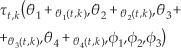
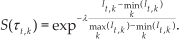
In Experiment 1, we restrict the robot shape to a straight line, with ϕ _i (i=1,2,3) = Orad. Four screw velocities θ _i (i.e., parameter vector U₁) are learned for this body shape and a given goal. Figure 3(a) shows the experiment for goal (−3m, −3m), the learning curves, and the changes in screw velocities during the learning.

Figure 3.

(a) Experiment 1 with a straight-line body shape: (i) Shows the robot reaching the goal position (−3 m, −3 m) (shown by the small blue circle) in a straight-line body shape. The final followed trajectory is indicated by the blue dashed line. (ii) The learning converges to the lowest cost for all 10 runs, taking around 20 updates for the average run (in bold). (iii) Shows that the learning of screw velocities stabilizes after the goal is reached at around 20 updates. The final values are θ₁ = −0.35rad/s, θ₂⁼ 0.77rad/s, θ₃ = −0.3rad/s, and θ₄ = 0.65rad/s. (b) Experiment 2 with a zigzag body shape: (i) Robot reaches the goal position (2m, −2m; the small blue circle), (ii) Learning converges to the lowest cost at around 16 updates for the average run (in bold red). (iii) The final learned screw velocities in the third picture are θ₁ = 0.16rad/s, θ ₂ = 0.61rad/s, θ₃ = 0.14rad/s, and θ₄ = 0.30rad/s.

4.2 Learning Robot Control for Any Fixed Shape

The experiment in this section demonstrates the learning of θ _i (i=1,2,3,4) when the robot has a different body shape. In Experiment 2, we fix the robot shape into a zigzag – with ϕ₁=0.5rad, ϕ₂ = −0.5rad, and ϕ₃ =0.5rad – prior to learning. θ _i (i.e., parameter vector U₁) are then learned for this body shape and a given goal. Figure 3(b) shows the experiment for goal (2m, −2m), along with the learning curves.

4.3 Learning All Seven Robot Control Parameters

This experiment demonstrates that the robot learns all of its seven control parameters using U₂, θ _i (i=1,2,3,4) and ϕ _i (i=1,2,3) for locomoting toward a given goal. Figure 4 shows the learning curves for the goal (−1m, −3m).

Figure 4.

Experiment 3: Learning all seven locomotion control parameters, (a) Learned goal position (−1m, −3m) shown in the inset. Learning converges to lowest cost for all 10 runs, taking around 20 updates for the average run (in red). (b) The learned screw velocities are θ₁ = −0.39rad/s, θ₂ = −0-02rad/s, θ₃ = −0.32rad/s, and θ₄ = −0.08rad/s. (c) The learned joint angles are ϕ₁ = − 0.05rad, ϕ₂ = 0.11rad, and ϕ₃=0.02rad.

4.4 Learning Robot Control for Periodic Body Movements

This experiment demonstrates how the robot locomotes toward a given goal with learned screw velocities and joint angle phases, so as to have periodic body movements. The parameter vector learned is U₃. Figure 5 presents the experiment and shows the goal position (−2m, −2m), the learning curves, and the changes to the screw velocities, joint angles phases and joint angles during the learning.

Figure 5.

Experiment 4: Learning all seven locomotion control parameters with periodic body movements, (a) The robot reaches the learned goal position (−2 m, −2 m), shown in the inset. The final followed trajectory is indicated by the red dashed line. Learning converges to lowest cost for all 10 runs, taking around 15 updates for the average run (in bold). (b) Learning of the screw velocities (θ _i ) and joint angle phases (φ _i ) converges around 15 updates. The final learned values are θ₁ = −0.10, θ₂ = 0.53, θ₃ = −0.12, and θ₄ = 0.50; φ _i are φ _i = 0.6, φ₂ = −0.5, and φ₃ = −0.3. (d) The three learned joint angles φ _i following sinusoidal motion shifted in phase. It shows that ϕ₂ and ϕ₃ are almost in phase, while ϕ₁ leads them.

From the results of these experiments, we can see how PI² learns control parameters (joint angles and screw velocities) for different goals and body shapes, and thus generates periodic and nonperiodic motor primitives. We can also see that, in most of these cases, convergence in learning was reached and the motor primitives were achieved within 12–20 updates.

5. Generating Complex Behaviour with Motor Primitives

The above demonstrates how motor primitives can be generated. Some of them are shown in Figures 3(a), 3(b), 4(a) and 5(a). A reasonable number of motor primitives are stored to form a library, which can be used to handle a variety of situations. The primitives are described as: “moving straight in a straight configuration”, “moving straight in an arc robot shape”, “moving diagonally in a zigzag robot shape”, etc. Figure 6, taken as an example, shows the main motor primitives. A part of the formed primitive library is given in Table 2. The robot chains some of these primitives, in order to produce a sequence of behaviours in the real environment. Parameter interpolation and sensory feedback are employed to generate new locomotion behaviour.

Table 2.

The Motor Primitive Library

Primitive	Real robot behaviour
P 1 s	move at 135° with a straight shape
P 1 a	move at 135° with an arc shape
P 2 s	move at 90° with a straight shape
P 2 a	move at 90° with an arc shape
P 2 z	move at 90° with a zigzag shape
P 3 s	move 45° diagonally with a straight shape
P 4 s	move straight forwards with a straight shape
P 4 z	move straight forwards with a zigzag shape
P 4 pe	move at −90° with periodic body movements
P 5 s	move −45° diagonally with a straight shape
P 5 pe	move at −30° with periodic body movements
P 6 s	move at −90° with a straight shape
P 7 z	move at −135° with a zigzag shape
P 8 s	move straight backwards with a straight shape
P 8 a	move straight backwards with an arc shape
P 9	move at 90° with a semi-arc shape
P 10	move straight forwards with a semi-zigzag shape
P 11	move at 45° with a semi-zigzag shape
P 12	move at 90° with a semi-zigzag shape
P 13	move straight backwards with a semi-zigzag shape

Figure 6.

Generated Primitives: P₁ to P₈ give the generated robot behaviours with different body configurations. P₁ gives the robot behaviour to move at 135°; for a similar description of other primitives, refer to Table 2. G1 to G8 give the existing goals, and the red arrowhead indicates the robot's head.

5.1 Chaining of Primitives

Figure 7 shows a graphical representation of how primitives have been chained in this work. The primitives can belong to any robot shape or configuration, whether straight-line, zigzag, arc, etc. As an example, Figure 7 shows that the first primitive to move at 20° (m1) forward is chained with the second primitive to move at 70° (m2) forward, in order to reach position C. These primitives are followed by the third primitive, which moves at −70° (m3) downward, thus finally reaching the goal. Primitives are also chained and driven by sensory feedback as a reactive control mechanism. For example, in an environment with obstacles, multiple primitives are chained by sensory feedback to allow the robot to avoid the obstacles and reach a goal. Similar sensory feedback techniques, such as sensing joint angles, etc., can also be employed. In this way, chaining can be effectively used to obtain new robot behaviours for unknown situations.

Figure 7.

Graphical representation of the chaining of primitives to produce complex robot behaviours, to achieve multiple goals. The red arrowhead indicates the robot's head, m1, m2 and m3 are the three angles relative to instantaneous robot body orientation. Three required primitives are selected to take the robot from start position A to the goal, via B and C points. The red dashed line gives the trajectory.

5.1.1 Symbolic planning for automatic action chaining

Here, we present a symbolic planning approach (i.e., a STRIPS-like planner [32]) for generating a plan based on learned primitives. This is executed at the highest level of abstraction, as in a multilayer cognitive architecture [129, 30]. The planner searches for plans using a declarative knowledge representation and generates actions to instruct the robot to achieve desired tasks, like moving to a goal or avoiding an obstacle, etc. The list of primitives in the library, shown in Table 2, is used for the action definition. The planning domain definition consists of a list of predicates, actions and planning operators. Predicates are logical formulas which take true or false values. In our example, the predicates are defined as

$1.ongoal(robot)2.obstacle(angle)$

The predicate ongoal(robot) describes the situation in which the robot is on the goal, whereas obstacle(angle) refers to a situation in which an obstacle is detected in the direction specified by the angle. In our case, angle ɛ {angletoGoal, angletoGoal + 90°, angletoGoal −90°}. An action is defined as move(angle, shape) to instruct the robot to move in the direction specified by the angle, with a given robot body shape. Planning operators (POs) consist of three parts: PO = {a, p, e}, with a = actions, p = preconditions, and e = effect. If p (a set of predicates) are true, then the corresponding PO can be applied using a, so as to act in order to produce the effect e. The change after execution is also coded as a set of predicates.

For the execution of a specific task, we need to define the planning problem, consisting of an initial state S_ini and the goal specification g. In our example, S_ini is defined as {ongoal(robot), obstacle(angletoGoal), obstacle(angletoGoal + 90°), obstacle(angletoGoal − 90°)}, i.e., a set of initial predicates at the start, with each taking true/false values. In turn, g is defined as the specification that ongoal(robot) = True, i.e., the final grounded predicate at the end of the task. In our case, we adopt a replanning strategy. The high-level planning module makes an evaluation at every action interval. If there is a violation of the preconditions (p) of the POs, while the effects (e) have not been yet obtained, then the system generates a new plan, with a replanning approach. Thus, the planner uses all the above elements to generate a sequence of actions, which produces the sequence of changes necessary to obtain g from S_ini. In Section 6, an example is presented of a plan to avoid obstacles.

5.2 Parameter Interpolation

Once this basic primitive set of P₁ to P₈ was selected, as depicted in Figure 6, this work made use of parameter interpolation of nonperiodic primitives, in an attempt to further generalize locomotion generation. The goal was to make the robot generate new motor controls, and actions necessary to reach new goals, from existing primitives.

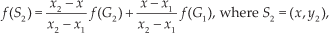
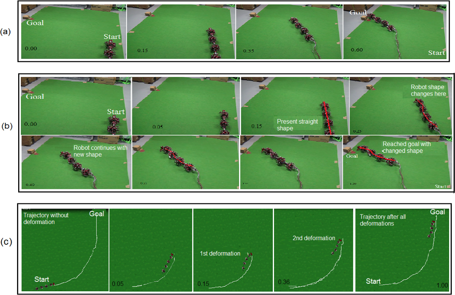
Here, bilinear interpolation – a basic interpolation method for non-linear systems – is used for interpolating parameters, considering that the snake-like robot follows nonlinear kinematics and uses all seven control parameters for interpolation. For interpolation, new goals are present in one of the quadrants marked as A, B, C and D, as shown in Figure 6. For example, by interpolating the learned control parameters for primitives P₁, P₂ and P₈ in the quadrant marked A, the motor control for the robot to move 120°, i.e., diagonally backwards to its start position, is generated. Similarly, to obtain new robot behaviours for new goals in the quadrant marked B, P₂,P₃ and P₄ are used for the interpolation; in the quadrant marked C, P₄,P₅ and P₆ are used; and in quadrant D, P₆,P₇ and P₈ are used for interpolation. Once the new goal has been mapped to see in which quadrant of the coordinate plane it belongs, and the necessary primitives have been selected, the corresponding learned parameters for the primitives are selected to give U_Pi for each one, with i being the primitive index:

$U_{P_i}=\left[{\dot{\theta }}_1\mathrm{,}{\dot{\theta }}_2\mathrm{,}{\dot{\theta }}_3\mathrm{,}{\dot{\theta }}_4\mathrm{,}{\varphi }_1\mathrm{,}{\varphi }_2\mathrm{,}{\varphi }_3\right]\mathrm{.}$

(15)

In this work, for convenience, we take each quadrant to be a 2m × 2m area, to help generate motor primitives. Thus, the interpolation is considered within this range. So, the total area covered by all quadrants of the coordinate plane comprises a 4m × 4m grid. For example, let the parameter interpolation set up take place in the quadrant marked as A in Figure 6. The goals G1,…,G7,G8 correspond to positions (2, 2), (0, 2), (−2, 2), (−2, 0), (−2, −2), (0, −2), (2, −2) and (2, 0), respectively. All goal positions are in metres (m). So, P₁, P₂ and P₈ are to be interpolated in A, thus giving i=(1, 2, 8) for Equation (15). As a result, the interpolation takes place with f (G2)=U_P2, f (G1)=U_P1, f (G8)=U_P8, f (O)= [0,0,0,0,0,0,0], with f giving the mapping between the learned goals and the required primitives. Positions G2=(x₁,y₂)=(0,2),G1=(x₂,y₂)=(2,2),G8=(x₂,y₁)=(2,0),O =(0,0). Thus, the interpolated parameters for a new goal G(x,y) are obtained as follows:

$f(S_1)=\frac{x_2-x}{x_2-x_1}f(O)+\frac{x-x_1}{x_2-x_1}f(G_8)\mathrm{,}\mathrm{where}{S}_1=(x\mathrm{,}{y}_1)\mathrm{,}$

(16)

$f(S_2)=\frac{x_2-x}{x_2-x_1}f(G_2)+\frac{x-x_1}{x_2-x_1}f(G_1)\mathrm{,}\mathrm{where}{S}_2=(x\mathrm{,}{y}_2)\mathrm{,}$

(17)

$f(G)=\frac{y_2-y}{y_2-y_1}f(S_1)+\frac{y-y_1}{y_2-y_1}f(S_2)\mathrm{.}$

(18)

In this way, new robot behaviours are obtained through interpolation from the elementary primitive set. An experiment is shown in Figure 8 to demonstrate this. Three primitives from Table 2 (P_1s, P₁₂, P₁₃) are interpolated in order to obtain a new robot behaviour (new control parameters), using Equations (16–18) for the new goal (2m, 1m), as shown in Figure 8(d).

Figure 8.

Experiment 5: Generating new behaviours with parameter interpolation. Start position is (0m, 0m). (a) Primitive P_1s from the library. It is generated using the goal (2m, 2m) for a straight-line shape. (b) Primitive P₁₂ from the library, which is generated using the goal (0m, 2m) for a semi-zigzag shape, having ϕ₁ = 0.5rad, ϕ₂ = −0.5rad, and ϕ₃ = −0.1rad. (c) Primitive P₁₃ from the library, which is generated using the goal (2m, 0m) for a semi-zigzag shape, (d) The robot reaches the goal (2m, 1m) using parameters obtained by interpolating the above primitives belonging to different robot shapes.

6. Experiments for Complex Tasks

This section presents Experiments (6–10), demonstrating how the robot handles complex tasks – like goal-directed obstacle avoidance, goal-directed locomotion with body deformation, and tasks with multiple goals – using the developed framework. We encourage readers also to view the supplementary video of these experiments, available at http://manoonpong.com/IJARS2015/svideo.mpeg.

6.1 Goal-Directed Locomotion with Obstacle Avoidance

The experiments in Figure 9 show goal-directed locomotion with and without obstacles. Figure 9(a) shows the experiment without any obstacles; here, the robot uses only one motor primitive (taken as Set 1) to reach the goal (−3m, −1 m). Set 1 consists of θ₁ = −0.26rad/s, θ₂ = 0.42rad/s, θ₃ = −0.29rad/s, and θ₄ = 0.34rad/s; and ϕ₁=0.05rad, ϕ₂=0.16rad, and ϕ₃= −0.02rad. Figure 9 (b) shows the experiment with obstacles. The obstacles are avoided here by sensing through an IR sensor attached to the robot's head. To achieve this, three robot behaviours are sequentially chained for avoiding obstacles and moving to the goal. From the primitive library in Table 2, two motor primitives - P₂ (which makes the robot move left, i.e., to 90°) and P_6s (which makes it move right, i.e., to −90°) – are selected and used. The robot starts with a learned parameter set (i.e., Set 1) for reaching the original goal (−3m, −1m). The IR sensor provides feedback on the distance between the obstacle and the robot. Once the robot has detected the obstacle (i.e., the IR signal is higher than the threshold), it automatically selects a predefined motor primitive (i.e., P_2s for moving to the left), so as to avoid the obstacle. Once the obstacle has been avoided (i.e., the IR signal is smaller than a threshold), the robot then returns to its previous motor primitive (i.e., moving straight towards the goal with Set 1). Following a predefined time-out period after moving straight, it then selects another motor primitive (i.e., P_6s moving to the right) and finally reaches the goal. In this way, the primitives are chained and activated using the sensor and a time-out period mechanism.

Figure 9.

Experiment 6: Goal-directed locomotion of the real robot without and with obstacles in a complex environment. (a) Real robot experiment without obstacles, showing the robot reaching the goal (−3m, −1m) using the learned control parameters. Start position is (0m, 0m). (b) Goal-directed obstacle avoidance behaviour in a real robot experiment. The robot reaches the goal (shown in red) while avoiding obstacles on its path. The robot behaviour is driven by chaining three motor primitives, obtained through PI².

Another experiment in obstacle avoidance is also shown in Figure 10. Two primitives – P_4s (to move straight) and P_2z (to move left) – are selected from Table 2 and chained, again using the IR sensor attached to the robot's head. The P_4s primitive is used by the robot when there is no obstacle detected (i.e., the IR signal is lower than a threshold) and P_2z as soon as an obstacle is sensed.

Figure 10.

Experiment 7: Real robot experiment demonstrating obstacle avoidance. All primitives are sequenced using IR sensory feedback. The numbers of the obstacles are marked; two obstacles can be seen being avoided at the shown timestamps.

However, further sensors can be added to render the locomotion fully sensor-driven. Additionally, a planner that analyses the scene (as far as is visible) and then automatically selects motor primitives to approach the goal and/or avoid obstacles can be implemented (as an additional module in the framework), using any planning method or reactive/proactive control method [31]. An example planner is presented below.

6.2.2 A symbolic planning example using primitives

Here, we briefly show an example of how a STRIPS-like planner [32] could be used to generate a plan (see Section 5.1.1). The task at hand is obstacle avoidance. The POs for this task (in terms of (a,p,e)) are defined in Table 3. Here, T shows that the predicate takes a “True” value, and F, “False”. With the move(), the corresponding primitive (e.g., P_2s and P_5s, in the case of the example shown in Figure 9(b)) is selected from Table 2 for action grounding: PO₁ takes the robot straight, PO₂ takes it left, and PO₃ takes it right.

Table 3.

Planning Operators for Obstacle Avoidance

	Definition
PO 1	a: move(angletoGoal, shape)
	p: obstacle(angletoGoal) = F, ongoal(robot) = F
	e: ongoal(robot)= T
PO 2	a: move(angletoGoal+90°, shape)
	p: obstacle(angletoGoal+90°) = F,
	obstacle(angletoGoal)= T
	e: obstacle(angletoGoal)= F
PO 3	a: move(angletoGoal-90°, shape)
	p: obstacle(angletoGoal-90°)= F,
	obstacle(angletoGoal)= T
	e: obstacle(angletoGoal)= F

To show how these operators can be searched and sequenced, the initial scenario shown in Figure 9(b) is taken. For this scenario, the starting state S_ini is {F,F,F,F}, and accordingly, a plan is generated consisting of a single PO: PO₁ At the point where an obstacle is detected, a replanning operation is performed with the new initial state S_ininew {F,T,F,F}. The new plan to reach the goal is then PO₂,PO₁ Alternatively, at the point of the obstacle, PO₃,PO₁ would also be a possible new plan, as can be ascertained from the p in Table 3 and from S_ininew. Similarly, for the initial setup in Figure 10, a plan PO₁ is generated at the start. When Obstacle 1 is detected, replanning occurs with S_ininew= {F,T,F,T}, and the new plan is PO₂,PO₁. As, S_ininew is again {F,T,F,T} when Obstacle 2 is detected, the new plan is again PO₂,PO₁, which thus allows the robot to reach the goal while avoiding the obstacles. In this way, a planner that uses the learned primitives obtained by PI² can be integrated into the framework for goal-directed locomotion.

6.2 Goal-Directed Behaviour with Multiple Goals

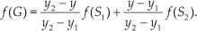
Here, the goal-directed behaviour of the robot is demonstrated as it is made to move through multiple goals. Figure 11 shows an experiment in which the robot moves through multiple sub-goals (G1 and G2) in order to reach the final goal (G3). Three primitives (P_1s,P_4z,P₉) are manually selected from Table 2 for this task, and their final chaining sequence is P_1s → P_4z → P₉. The chaining can be described as follows: the robot uses P_1s, the motor primitive for moving to 135 with a straight-line shape, to reach the first goal (G1) from the start; this is followed by P_4z, for moving straight with a zigzag shape, to reach the second goal (G2); finally, the robot uses P₉, for moving to 90° upward with a semi-arc shape, to reach the final goal (G3). Another multiple goal experiment is shown in Figure 12. Primitives of different shapes, and both nonperiodic and periodic, are selected in these experiments to demonstrate the possibility of chaining between different robot configurations.

Figure 11.

Experiment 8: Real robot movement through multiple goals. The followed trajectory is indicated by the dotted lines and the goals are marked in red. The robot reaches the final goal via G1, G2 and G3. The three motor primitives giving the three control parameter sets are sequentially activated.

Figure 12.

Experiment 9: The robot reaches multiple goals (G1, G2, G3), which are marked. The chaining of the robot behaviours is IM₁ → IM₂ → IM₃ → P_5pe → P_4pe IM₁ (obtained from interpolating P_8s, P_1s and P_2s), which gives the robot behaviour for moving to 120° diagonally in a straight shape, is chained with IM₂ (obtained from interpolating P₁, P₂ and P_8s). This is followed by IM₃ (obtained from interpolating P_4a, P_5s and P_6a), for moving the robot to −30° with a bent arc-like configuration, with all its joint angles negative. IM₃ is used to change the robot's direction. In this way, G1 is reached. To reach G2, the motor primitive P_5pe for moving to −30° diagonally with periodic body movements is used. In order to reach the final goal (G3), P_4pe, for moving the robot to −90° vertically downward with periodic body movements, is used.

6.3 Goal-Directed Locomotion with Body Deformation

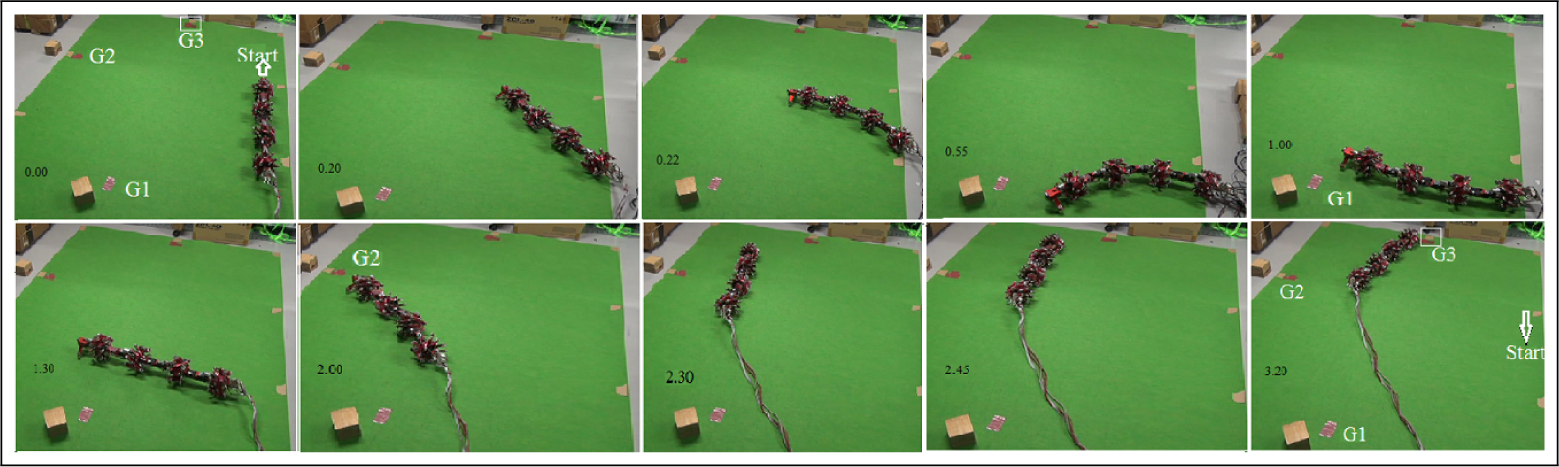
In these experiments, the robot successfully moves toward a goal even when it has suffered body deformation, i.e.; changes to its body shape, on its way. A single deformation is shown in Figure 13(b), whereas Figure 13(c) shows multiple deformations in body shape.

Figure 13.

Experiment 10: Goal-directed locomotion while handling changes in body shape. (a) Robot reaches the goal without deformation, maintaining ϕ _i =0rad throughout its locomotion. The goal is (−1m, 2m) and the start position (0m, 0m).(b) Even when its body shape changes on its path at 0.25min, it continues with the new shape to reach the same goal (−1m, 2m). It uses the corresponding motor primitives/robot control for the new body shape to handle this change. (c) Simulation showing that the robot can successfully handle multiple body shape changes on its route, and still reach the goal. The first snapshot shows the robot reaching the goal (−2m, 3m) by moving at 60°, without any deformation and maintaining ϕ _i =0rad throughout. Two deformations – the first from a straight to an arc shape, followed by a change to a semi-zigzag (at both instants, the robot going to 20°) – are handled using two derived motor primitives, as shown in the second snapshot onwards. The pictures also show how the trajectory (the white line) is maintained even when there is deformation. This points to a systematic primitive library formation, which can be used as required.

Figure 13(a–b) uses three motor primitives - P₁₀, P₁₁, P₁₂ - which are manually selected from Table 2 for the task. Figure 13(a) shows the robot behaviour when there is no deformation on its way to the goal (−1m, 2m). The learned parameters for this situation, taken as Set 1, are θ₁ = −0.38rad/s, θ₂ = −0.05rad/s, θ₃ = −0.42rad/s and θ₄ = 0.06rad/s, with ϕ₁ =ϕ₂ =ϕ₃ =0. Figure 13(b) shows the robot behaviour when its body shape changes on the way toward the goal (−1m, 2m), while it is using the above Set 1 parameters. When it detects a change in its body shape, using its joint angle sensors, it uses another robot behaviour, IM₄, to enable it to handle this morphological change. IM₄ (belonging to the semi-zigzag robot shape of ϕ₁ = 0.5rad, ϕ₂ = −0.5rad, and ϕ₃ = −0.1rad) is generated using parameter interpolation of the primitives P₁₀, P₁₁ and P₁₂, in order to move to 30°. The interpolation is performed following Equations (16–18). The primitives to be interpolated are selected based on the new deformed robot shape and the angle to the goal at the instant that deformation takes place. Interpolation is used to generate new behaviours, as no suitable primitive previously existed. Using the derived behaviour IM₄, the robot moves with this new semi-zigzag shape and is able to finally reach the goal.

7. Conclusion

We have successfully developed a framework that provides a model-free goal-directed locomotion controller for a snake-like robot with screw-drive units. The framework handles a large number of behavioural cases (within a defined scope). With the complete framework for generating motor primitives using PI², along with parameter interpolation and the chaining of primitives and/or interpolated parameters, the robot can successfully perform goal-directed locomotion in different situations. The framework thus generalizes the locomotion generation for the complex nonstandard snake-like robot.

Real robot experiments show that using the complete framework enables the robot to successfully handle challenging tasks like reaching a single/multiple goal(s) while avoiding obstacles or compensating for a morphological change (such as body damage) during locomotion. Furthermore, it has also been shown that, by learning a proper combination of locomotion control parameters (i.e., screw velocities and joint angles using PI²), motor primitives can be generated in a numerically simple manner. Proper control parameters were also found for when the robot was configured with different shapes (i.e., straight-line, zigzag, arc, etc.) or with periodic body movements, thereby establishing a rich primitive library which could then be used. Thus, this framework and approach solves the coordination problems relating to such a high degree-of-freedom system as this nonstandard snake-like robot. As a result, the robot is able to reach a given goal in different situations. In addition, this study also shows how PI² can be used to learn motor control for this type of nonstandard snake-like robot.

In some of the real robot experiments, a small deviation (i.e., approximately 25cm) from the goal was observed. This deviation was due to real conditions, such as friction, cabling, etc. Major changes, like the variation of the friction coefficient, can be handled by relearning the existing motor primitives. However, sensory signals (e.g., joint angles, goal detection, slip detection, etc.) are required in order to enable the robot to perform online learning autonomously, which can then adjust or optimize the parameters of our motor primitives to deal significantly with body and environmental changes. Implementing such sensors with online learning is one of our future plans.