Sage Journals: Discover world-class research

Abstract

This paper presents a novel approach to discovering motor primitives in a hierarchical database of example trajectories. An initial set of example trajectories is obtained by human demonstration. The trajectories are clustered and organized in a binary tree-like hierarchical structure, from which transition graphs at different levels of granularity are constructed. A novel procedure for searching in this hierarchical structure is presented. It can exploit the interdependencies between movements and can discover new series of partial paths. From these partial paths, complete new movements are generated by encoding them as dynamic movement primitives. In this way, the number of example trajectories that must be acquired with the assistance of a human teacher can be reduced. By combining the results of the hierarchical search with statistical generalization techniques, a complete representation of new, not directly demonstrated, movement primitives can be generated.

Keywords

Imitation Learning Motor Primitives Trajectory Databases Hierarchical Graph Search

1. Introduction

In contrast to robot manipulators used in industry, autonomous robots working in domestic environments are not expected to repeat the same task with the same movements over and over again. Since the tasks and related conditions change constantly, manually programming the movements for every variant of a given task is not feasible. One of the most successful and widely used approaches to the acquisition of new sensorimotor behaviours is learning by imitation (or programming by demonstration) [1, 4, 23]. In such systems, initial movements are acquired by observing a human demonstrating a task. The demonstration is often captured using magnetic or optical marker-based systems. Such an approach has been utilized to replicate hard-to-program movements, such as dancing [26, 20, 19]. Research on markerless, vision-based systems for human tracking has also become a thriving area [18] and has seen a lot of success with the advent of low-cost RGB-D cameras [24]. Alternatively, a human can physically guide the robot to perform the desired movement via kinaesthetic teaching [7], which has the advantage that the captured movement is already adapted to the robot's kinematics and dynamics.

An aspect of research on imitation learning focuses on learning from a single demonstration, such as, for example, in the case of dynamic movement primitives (DMPs) [8]. Hidden Markov models [9] are another popular representation for the encoding of movement primitives. Multiple demonstrations have been used, for example, by Forte et al. [6], where a set of example trajectories was generalized with local regression methods to synthesize a trajectory that solves the task in a new situation within the trajectory training space. For this approach to work, the trajectories must transition smoothly between each other as a function of the parameters describing the task. Multiple demonstrations were also encoded with Gaussian mixture models [2, 10]. Alternatively, reinforcement learning was applied to generalize motor primitives for new situations by Kober et al. [12]. The need to acquire numerous demonstrations in order to generalize example trajectories for new situations is one of the major stumbling blocks in the practical application of imitation learning systems.

Compared to the work in the computer graphics community - which has always assumed that a large database of diverse motion data is available for the generation of computer animations - the number of example movements considered in robot programming by demonstration research has usually been much more limited, and the example trajectories have been less diverse. The work of Kulić et al. [15, 14] is a notable exception. They used hidden Markov models for incremental learning and the hierarchical organization of motion primitives, but they do not focus on discovering new movements in these data. In contrast, the computer graphics community has shown that, by exploiting the structured nature of motion capture data - which is made evident in motion graphs - smooth transitions between interconnected body movements can be found [21]. Motion graphs were proposed to encapsulate connections in the available motion capture data. They were applied by Kovar et al. [13] to generate different styles of locomotion along arbitrary paths. Their graph search algorithm was able to find nodes which represent possible transitions between parts of the captured movements. Motion graphs and interpolation techniques were combined by Safonova and Hodgins [22] in order to increase the number of paths through a graph. While the motion graph literature is vast, our work is most closely related to the approach of Yamane et al. [27], who used binary trees to organize the data and the resulting transition graphs in order to generate human body locomotion on a desired path. Sidenbladh et al. [25] also use a binary tree structure for the efficient sampling of human poses.

This paper proposes an approach that uses the concept of motion graphs, binary trees and a hierarchical search to generate new movements that were not directly demonstrated by the teacher. In this way, the number of human demonstrations needed to synthesize new movements can be reduced. New example trajectories are generated through a graph search, which can be used by statistical generalization [6] to create new movement primitives for arbitrary configurations.

Initial demonstrated example movements are organized in a hierarchical graph-like structure. State vectors, encoding demonstrated movements, are clustered using the k -means algorithm [16], as it was shown to be most efficient for our approach. The results of clustering are used to construct a binary tree, which represents the captured data at different levels of granularity. Every level of the binary tree is associated with a transition graph that describes transitions between the nodes at that level. The nodes contain state vectors from all example trajectories. The database is used to find new connections between nodes and thus new movements. If the path at the desired level does not exist, a top-down hierarchical database search is employed in order to find optimal partial paths. Dynamic movement primitives are used to combine them into smooth and continuous trajectories from the given start and end state vectors at the desired level of granularity. Statistical methods [6] are then utilized to generalize the newly discovered sets of trajectories and to create a complete representation of a newly discovered movement primitive.

While other works relating to motion graphs synthesize new movements through a graph search and/or interpolation, we employ a hierarchical partial paths search, which enables us to synthesize new movements by finding partial paths at lower levels of granularity. With this, we generate movements at desired levels of granularity while avoiding big parts of movements stemming from interpolation, which would reduce the similarities to demonstrated movements and in turn reduce the needed precision for, inter alia, manipulation tasks.

The rest of the paper is organized as follows. In Section 2, we present the process of constructing the database. The next section is divided into three parts; Subsection 3.1 deals with path searches in transition graphs, Subsection 3.2 with hierarchical searches of partial paths, and Subsection 3.3 with time evolution and DMPs. Section 4 presents the statistical generalization of the newly discovered sets of movement trajectories. The experimental evaluation of our approach is given in Section 5, while the discussion and conclusion are given in Section 6.

2. Generation of a hierarchical database of example movements

The example trajectories can be acquired either in the task or in the joint space. For the purpose of building the database, we concatenate the acquired trajectories in a sample motion matrix,

Y = [y_{1}, y_{2}, \dots, y_{n}],

(1)

where y _i denotes the state vectors sampled at a given discrete time interval and n is the total number of all postures belonging to all of the example trajectories incorporated into the database. State vectors for the end-effector trajectories specified in Cartesian space can, for example, be defined as

y_{i} = {[p_{x i}, {\dot{p}}_{x i}, p_{y i}, {\dot{p}}_{y i}, p_{z i}, {\dot{p}}_{z i}]}^{T},

(2)

where p_ji and ${\dot{p}}_{j i}$ , $j = x, y, z,$ denote the position and velocity at time t_i. If the trajectories are given in the joint space, then the state vectors can be defined as

y_{i} = {[q_{1 i}, {\dot{q}}_{1 i}, q_{2 i}, {\dot{q}}_{2 i}, \dots, q_{d i}, {\dot{q}}_{d i}]}^{T},

(3)

where the j -th joint angle and its velocity at time t_i are denoted by q_ji and ${\dot{q}}_{j i}$ , and A is the number of the robot degrees of freedom (DOFs).

Once example trajectories are stored and arranged in a sample matrix, they can be utilized to build a binary tree. The complete sample data matrix Y represents the root node v₁¹, i.e., the first node at the first level, which we split and thus acquire its two child nodes at the second level, v₁² and v₂². As each node is associated with a cluster of state vectors, splitting is done by a clustering algorithm. We use k -means clustering algorithm (with k = 2) as it shown to suit our needs best (see Subsection 5.2). The data in each of these nodes are then split again to acquire nodes at the next depth of the binary tree, as seen in Fig. 1. The division into two child nodes (i.e., the binary tree) was selected to generate a representation of sample movements on as many different levels of granularity as possible. This is useful for finding and joining partial movements in the database, as will be explained in Section 3.

Figure 1.

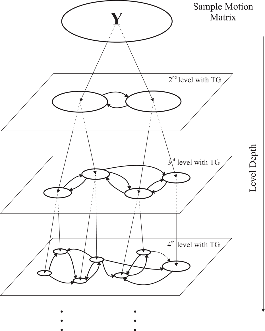
Generation of the hierarchical movement database with binary tree and transition graphs. The figure shows the structure of our database. The sample motion matrix Y is divided into two child nodes with k-means clustering. Then, the transition graph (TG), which represents probabilistic transitions between the nodes at this level, is built. The data associated with each node is then clustered into child nodes for the 3^rd level, where the TG is built again. We continue this procedure until all nodes fit the stopping criteria. Note that we expand those nodes to the last level and thus represent all the data at all the levels.

A criterion based on the variability of the data contained in the node is used do decide when to stop splitting the tree nodes. We define the mean distance d_v of node v as

d_{v} = \frac{\sum_{i = 1}^{n_{v}} d (y_{v i}, c_{v})}{n_{v}},

(4)

where n_v denotes the number of state vectors clustered at node v. The Euclidean distance d( y _vi, c _v) is determined between the state vector y_vi associated with node v and the node's centroid c_v, which is calculated by the k -means algorithm. If d_v is lower than a predefined threshold, then the state vectors contained in the node are deemed to be similar. By not splitting the nodes in this case, we avoid new nodes that would make the binary tree unnecessarily deep. However, we split the nodes even if they include a small number of state vectors if these state vectors are sufficiently diverse. In this way, we gain the precision of our representation while preventing the binary tree and the resulting transition graphs from becoming unnecessarily large. With this criterion, we cluster the data into nodes until we do not have any nodes remaining to split. We extend every branch to the last level by copying the leaf nodes, thereby ensuring that all the state vectors are represented at all levels of the binary tree.

At each depth level of the binary tree, we build a transition graph that represents all the transitions between the nodes at the current depth (see Fig. 1). The edge weights in the transition graph represent the probability of transition from one node to another. The transition probability from node v_k to node v_l is estimated by

Φ_{k l} = \frac{m_{k l}}{n_{v_{k}}},

(5)

where n_vk denotes the number of state vectors clustered at node v_k and m_kl denotes the number of transitions observed in all the trajectories of the original data, i.e., all the state vectors clustered in node v_k that have a successor in node v_l.

To accelerate processing we compute the mean x_v of the position components of all the state vectors y_vi associated with node v. Only if the node contains exactly one final configuration on an example trajectory do we store this final configuration instead of the position mean of all the state vectors. In this way, we ensure that the movements generated by the graph search end in the same end points as the original movements. By combining several trajectories in the same node, we lose the time component. We will explain later on in Section 3.3 that the time duration t_v of each node v is estimated through a ratio of the number of state vectors associated with node v and the number of original example trajectories passing through it.

3. Discovering new trajectories

Given the binary tree, the means of the state vectors x _v (or end points) at node v of the binary tree, and the transition graphs TG for every level l, we can now search for new sets of example movements in the transition graphs and thus expand the initial database of example movements (see Figure 2, sub-parts 2a, 2b and 2c). We do this by utilizing a transition graph search at the desired level ld. If no paths are found, we employ a hierarchical partial paths search. The (partial) paths are then enhanced by time evolution and encoded as DMPs. For clarity, we limit the following discussion to Cartesian space trajectories; joint space trajectories could be treated equivalently. Alg. 1 describes the process of finding a new example movement, while Alg. 2 focuses on a hierarchical search of partial paths (Subsection 3.2 and Fig. 2, subpart 2b).

Figure 2.

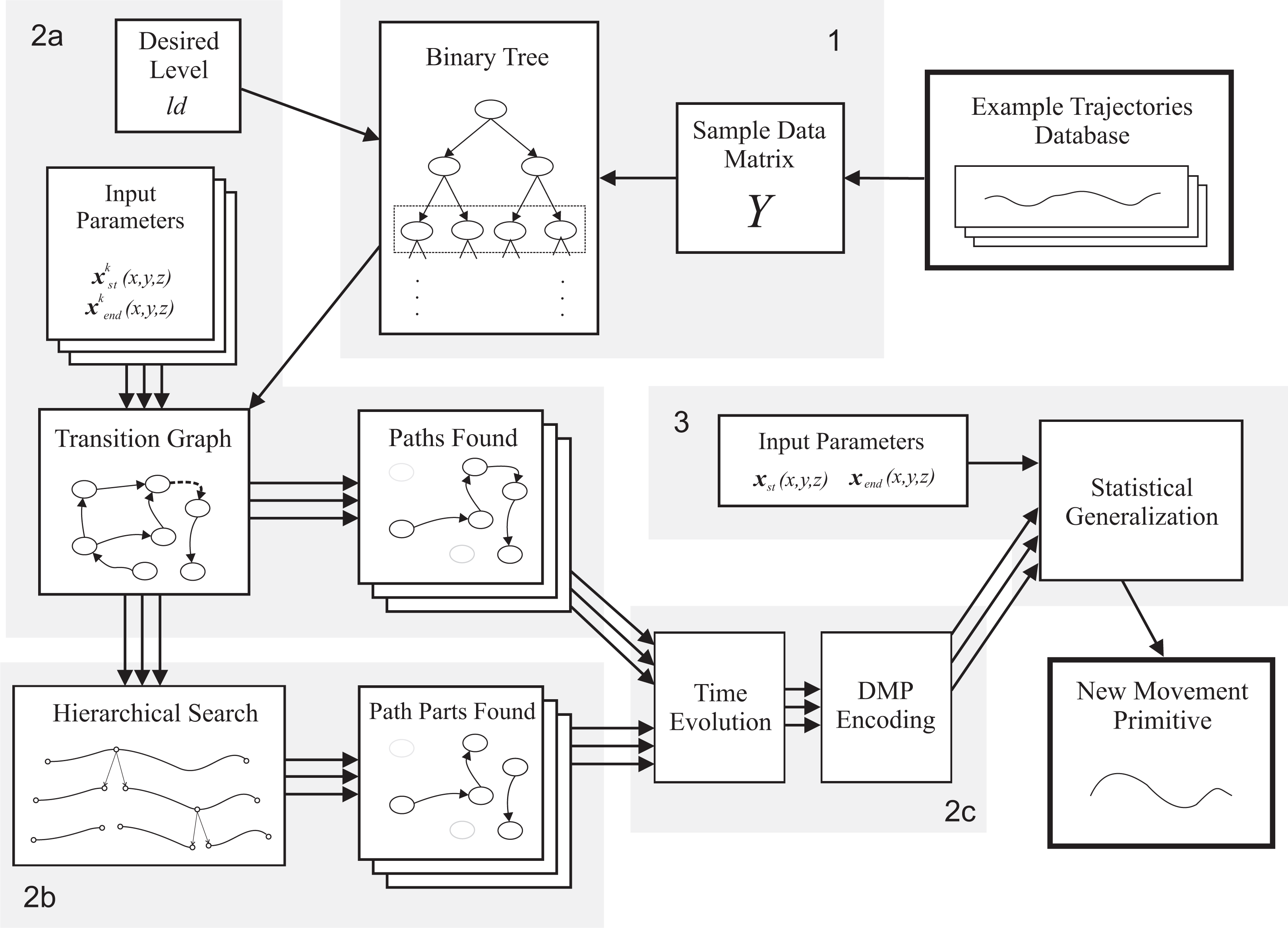
A block diagram presenting the proposed approach. 1) Building the hierarchical database. Captured example trajectories are stored in sample data matrix Y . It is used as a root node, which is clustered into two child nodes. These are then clustered further to obtain the nodes at the next level. At each level a transition graph (TG), which encodes probabilistic transitions between the nodes at this level, is constructed. We continue this process till the last level. 2a) Transition graph search. Desired start and end positions and the desired level of the database is selected. Nodes closest to the desired positions in the TG at the specified level of the database are found. A^* search algorithm is applied to find possible shortest paths. If the desired start and end nodes belong to the same connected component in the TG, desired paths are found. 2b) Hierarchical search. The hierarchical structure of the database is used to find partial paths. These parts are used to connect desired nodes at the desired level of the database. 2c) Time and DMPs. Newly found paths and/or partial paths are enhanced by time evolution and encoded as dynamic movement primitives. 3) Statistical generalization. Statistical methods can now be utilized to generalize the newly discovered sets of movements and obtain a complete representation of a new movement primitive.

3.1 The transition graph search

We start the process of discovering new discrete movement primitives (i.e., point-to-point movements such as reaching or grasping) by selecting the desired start and end points x _st and x _end of the movement. If the desired start and end points are not among the computed position means, we first establish the closest start and end nodes v_st^ld and v_end^ld in the transition graph at the desired level ld. The desired level determines the fidelity of any reproduction compared to the original trajectories. Normally, we select the last level in the binary tree, since here the degree of accuracy is highest. In the simplest case, when the start and end nodes belong to the same connected component of the transition graph, we can find a path P^ld (v_st^ld, v_end^ld) between these two nodes by using the A^* algorithm. A path is a series of nodes

P^{l d} (v_{s t}^{l d}, v_{e n d}^{l d}) = {v_{s t}^{l d}, v_{2}^{l d}, v_{3}^{l d}, \dots, v_{e n d}^{l d}},

(6)

connecting start and end nodes in the transition graph at level ld. If this is not the case, we need to find partial paths connecting the nodes (Tine 2 in Alg. 1 and Fig. 2), using the proposed hierarchical search.

Algorithm 1: Searching for new example movement Input: Desired start and end point x_st and x_end, respectively, and the desired level ld of the hierarchical database Output: New discovered trajectory nTrj encoded as a DMP 1 Find nodes v_st^ld and v_end^ld on level ld closest to desired start and end points x_st and x_end 2 P^ld = Find Partial Paths(v_st^ld, v_end^ld, ld) 3 Transform the discovered partial paths specified as a sequence of graph nodes at level ld into corresponding mean values of position parts of state vectors {x_i} and their time evolution T_i 4 Interpolate (and combine) the resulting sequence of position state vectors by encoding it as DMP and thus gain nTrj 3.2 The hierarchical search

If the desired start and end nodes are not connected in the transition graph - which can happen especially if the start and end points do not belong to the same trajectory - at the desired level, we take advantage of the hierarchical structure of the binary tree to find partial paths that would connect them (Alg. 2 and Fig. 2, subpart 2b). First, we find the deepest level at which the transition graph has a connection between the nodes v_st^l and v_end^l that are associated with the desired start and end points x_st and x_end. Such a level always exists because there is only one node at the top level. This is done by moving up the levels and using the A^* search algorithm until a path P^l is found (Alg. 2, Lines 1–5). However, this higher level does not have the desired granularity. To achieve proper granularity, we need to move down to the desired depth ld. Since the desired path does not exist at the deeper levels, we need to find a series of partial paths {p P_i^ld} which connects the desired start and end nodes v_st^ld and v_end^ld at the desired level ld.

The hierarchical search for partial paths is outlined by a simple example in Fig. 3 and by pseudo-code in Alg. 2, Lines 7–20. The search is started by taking the path P^l at the lowest level l at which such a path exists. This means that, at the beginning, there is only one partial path. We then start moving down the levels, l = l + 1, and find all the child nodes of the border nodes of each partial path. We then apply A^* to find a connecting path, i.e., the paths between successive border nodes (Alg. 2, Line 12). If the direct connecting path at this level does not exist, then the nodes that broke the connection must be found. These are used to construct partial paths between the desired nodes (Alg. 2, repeat loop starting at Line 11). Once a series of partial paths that can be used to connect the start and end nodes at this level (i.e., v_st^l and v_end^l) has been found, we select the shortest connection between these two nodes (Alg. 2, Line 19 and Fig. 3). We continue moving down the levels and searching for partial paths until we reach the desired level l=ld. At this point, the discovered path connecting the desired start and end nodes is represented by a series of partial paths,

P^{l d} = {p P_{1}^{l d}, p P_{2}^{l d}, \dots, p P_{n_{l d}}^{l d}},

(7)

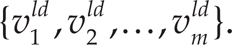
which can be translated into a sequence of nodes

{v_{1}^{l d}, v_{2}^{l d}, \dots, v_{m}^{l d}} .

(8)

Figure 3.

Hierarchical search of partial paths (see Alg. 2) illustrated by a simple example. After the path P^ld (v_st^ld, v_end^ld) was not found at the desired level of the database ld, the lowest level ld − 4, where a connecting path exists, was found. We then moved one level down to find connection at level ld − 3. As the direct connecting path at this level P^ld−3(v_st^ld−3, v_end^ld−3) did not exist, we searched for a node that broke the connection. A^* search was used in order to find the two partial paths. One connecting the start node v_st^ld−3 and one of the break node's children and the other connecting the other break node's child with the end node v_end^ld−3. We then move down another level to ld − 2 starting with the two partial paths. No new break points occurred at this level. When moving down one more level to ld − 1, it was not possible to connect the descending border nodes of the right partial path. New partial paths had to be found instead, so moving to the desired level ld resulted in three partial paths. The bottom of the figure shows DMP-based interpolation of partial paths into a smooth and continuous trajectory.

Algorithm 2:

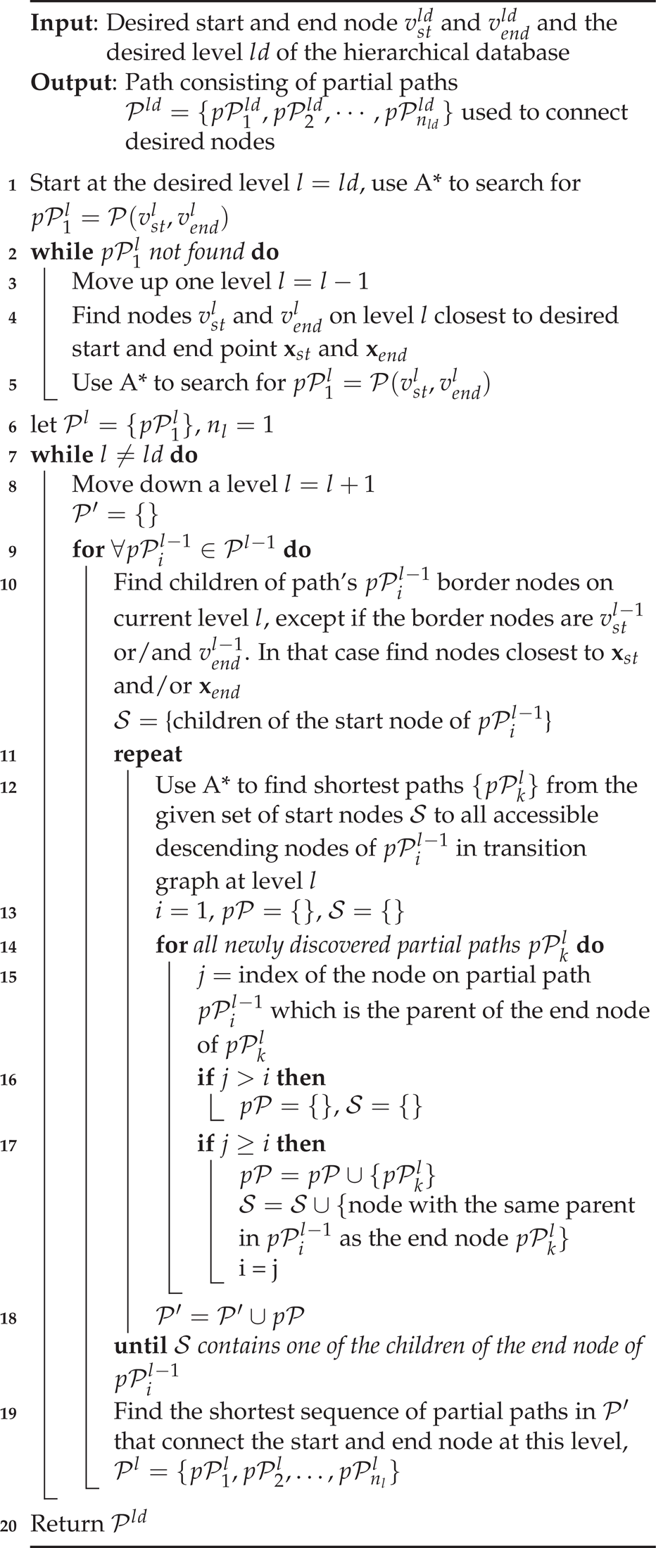
Hierarchical search for partial paths Find Partial Paths

3.3 Time evolution and DMP encoding

New example trajectories are defined by the positional means x _i of the sample points associated with nodes v_i^ld, i = 1, …, m, which need to be enhanced by time stamps. For this purpose, we define the duration of a single node v as follows,

t_{v} = \frac{n_{v}}{m_{v}} Δ t,

(9)

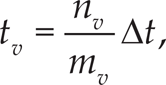
where 1/Δt is the sampling frequency, n_v denotes the number of state vectors clustered in node v, and m_v the number of trajectories passing through node v. The discovered trajectories can now be written as a sequence

M = {(x_{1}, T_{1}), (x_{2}, T_{2}), \dots, (x_{m}, T_{m})},

(10)

where

T_{i} = {\begin{array}{l} 0 & if i = 1, \\ \frac{t_{v_{i - 1}} + t_{v_{i}}}{2} & if i > 1. \end{array}

(11)

We encode each dimension of the discovered trajectory {( x ₁, T₁),( x ₂,T₂), …, ( x _m, T_m} as a DMP [8]. The DMPs are defined by the following nonlinear system of differential equations,

τ \dot{v} = K (g - y) - D v + f (s) .

(12)

τ \dot{y} = v .

(13)

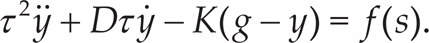
The linear part of Eqs. (12) – (13) ensures that y converges to the desired final configuration, denoted by “g”. The nonlinear part f(s) modifies the shape of a given movement and is defined by a linear combination of radial basis functions,

f (s) = \frac{\sum_{i = 1}^{N} w_{i} ψ_{i} (s)}{\sum_{i = 1}^{N} ψ_{i} (s)}

(14)

ψ_{i} (s) = \exp (- h_{i} {(s - c_{i})}^{2}),

(15)

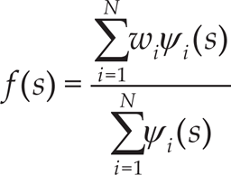
where ѱ_i defines the basis functions, with centres at c_i and widths of h_i > 0. As seen in Eq. (14), f (s) is not directly time dependent. Instead, the phase variable s defined in Eq. (16), with an initial value s(0) = 1, is used

τ \dot{s} = - α_{s} s .

(16)

The phase is common across all the DOFs or dimensions. By specifying the time evolution through the phase, it becomes easier to stop the clock in the case of external perturbations which cause the robot to deviate from the desired trajectory. It can be shown that - given the properly defined constants K, D, τ, α_s > 0 - the above system is guaranteed to converge on the desired final configuration g.

Eq. (12) – (13) can be rewritten as a second-order system,

F (T_{i}) = τ^{2} \ddot{y} (T_{i}) + D τ \dot{y} (T_{i}) - K (g - y (T_{i})),

(17)

By substituting y with the corresponding component of x _i and its derivatives ${\dot{x}}_{i}$ and ${\ddot{x}}_{i}$ at time T_i - here denoted by $y (T_{i}), \dot{y} (T_{i}), \ddot{y} (T_{i})$ - we can write our target function (17) as

F (T_{i}) = τ^{2} \ddot{y} (T_{i}) + D τ \dot{y} (T_{i}) - K (g - y (T_{i})),

(18)

where the goal value g is specified by the corresponding component of x _m. By defining

f = [\begin{matrix} F (T_{1}) \\ ⋮ \\ F (T_{m}) \end{matrix}], w = [\begin{matrix} w_{1} \\ ⋮ \\ w_{N} \end{matrix}],

(19)

we can write a system of linear equations

X w = f,

(20)

where

X = [\begin{matrix} \frac{ψ_{1} (s_{1})}{\sum_{i = 1}^{N} ψ_{i} (s_{1})} s_{1} & \dots & \frac{ψ_{N} (s_{1})}{\sum_{i = 1}^{N} ψ_{i} (s_{1})} s_{1} \\ ⋮ & ⋱ & ⋮ \\ \frac{ψ_{1} (s_{m})}{\sum_{i = 1}^{N} ψ_{i} (s_{m})} s_{m} & \dots & \frac{ψ_{N} (s_{m})}{\sum_{i = 1}^{N} ψ_{i} (s_{m})} s_{m} \end{matrix}],

(21)

with ѱ_i and s_i set according to (15) and (16).

By solving the above system, we gain the appropriate DMP weights w and thus learn the target function (18). By transforming (10) into a DMP, we ensure that combined partial paths result in a smooth and continuous trajectory and thus prepare the newly discovered movements for execution on a robot. The gaps between successive partial paths can be successfully bridged by DMPs, as shown below in Fig. 9.

Figure 4.

Our experimental setup. It consists of two Kuka lightweight robot arms, three fingered Barrett hand, two mounted cameras, and a shelving unit. The shelving unit consisted of six compartments, i. e. goal areas. The starting area on the table, where the object was put before each execution, is marked with blue lines.

Figure 5.

Vision error. Different positions across the starting area were determined by robot's forward kinematics and at the same time estimated by stereo vision. Blue dots represent positions obtained by forward kinematics, whereas the connected red dots represent the same object position as estimated by vision. Note that the z axis is scaled for better visibility. On the average the systematic vision error was 0.85 cm.

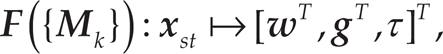
4. The generation of new movement primitives

Through a hierarchical graph search and DMP-based interpolation, we can connect the start and end configurations even if they do not belong to the same demonstrated movement. In this way, we can significantly increase the number of initial example movements {M_k), where the example movements are defined as in (10).

Figure 6.

Evaluation of clustering algorithms. Top graph shows Davies-Bouldin index values for each database level and each algorithm. Lower values represent better clusters. Similarly, the bottom graph shows Dunn index values, but with Dunn index, higher values represent better clusters.

But even if a large set of movements { M _k} is obtained, it is highly unlikely - at least in natural environments - that the exact desired movement can be found in the example set. To accomplish a task such as reaching towards and/or away from an object located at any position in the workspace, we need to generalize the discovered example movements for new reaching configurations, i.e., a new start x _st and end configuration x _end. This can be accomplished by means of statistical generalization, whereby a movement suitable for the current object configuration is synthesized from a number of example trajectories (Section 3 in Fig. 2).

Given the DMP representation and trajectory data expanded by the graph search { M _k}, we can generalize the example trajectories within the trajectory training space [6]. In the case of reaching movements, we use a methodology that learns a function

F ({M_{k}}) : x_{s t} \mapsto {[w^{T}, g^{T}, τ]}^{T},

(22)

where w, g and τ are the parameters that define a DMP, which starts in x _st and ends at the desired position in the workspace. The function F is learned as a combination of locally weighted regression and Gaussian process regression. For this method to work, the discovered trajectories M _k need to transition smoothly between each other as a function of the start and end configuration x _st or x _end. We omit the details and refer the reader to Forte et al. [6]. See also Section 5 for the experimental evaluation of this procedure.

5. Evaluation

We evaluated our approach in an experiment where a robot had to learn how to pick an object positioned anywhere in the starting area and put it on a desired shelf. The starting area was 62 cm by 76 cm in size. There were three levels of shelves and each of them was further divided into two parts. Each goal area could be reached through a 30 cm by 30 cm opening. Unless stated otherwise, data in Cartesian space were used, i.e., all the state vectors included in the hierarchical database are defined in Cartesian space (2). Two Kuka lightweight robot arms were used for the experiment: one for holding the stereo camera system used for vision and one for executing the task. Objects were grasped using a three-finger Barrett hand. They were easy to grasp and detect, as these issues are not the main subject of our research. The experimental setup can be seen in Fig. 4.

Figure 7.

Demonstration of reaching movements by kinesthetic guiding of the Kuka lightweight robot arm. From each of the six areas in the starting zone, 5 movements were demonstrated to a unique shelving unit part. The object was held with the Barrett hand and its starting position was estimated by stereo vision. The object did not collide with the shelving unit during the demonstration.

Figure 8.

Captured movements for the example database. The goal areas, i. e. the shelving unit is shown in black and gray. The trajectories of captured movements are shown in blue. The trajectory starting points are marked with red circles. From each of the six areas in the starting zone, 5 movements were captured to a unique shelving unit part. Altogether 30 movements were demonstrated and captured.

5.1 Vision evaluation

As stated before, the starting object positions were estimated by stereo vision. Some noise and errors are to be expected with such estimation despite accurate camera calibration. By comparison of the positions obtained by the robot's forward kinematics and stereo vision, we estimated the systematic vision error to be 0.85 cm. These positions, which roughly cover the starting area, can be seen in Fig. 5. The systematic vision error can in part be learned by Gaussian process regression, which is used for generalization. Since stereo vision is used to estimate the object's starting position in training and when generating new movements, the vision error is corrected by Gaussian process regression.

5.2 Clustering algorithm evaluation

Before building the binary tree database, we needed to select a clustering algorithm. We compared three popular and widely-used approaches by building our database from the captured movements, as explained in Section 2, and then evaluating clusters at each level. Two metrics were used, both of which were internal evaluating schemes. We evaluated the clusters by calculating Dunn [5] and Davies-Bouldin (DB) indices [3] at each level of the binary tree build by each of the three algorithms: k -means, PCA with the minimum-error thresholding technique, and expectation-maximization (EM) clustering [17]. The evaluation results are shown in Fig. 6. The top graph shows the DB index values for each database level and algorithm. Lower DB index values represent better clusters, as they define smaller distances between values in clusters and larger distances between cluster centres. It can be seen in the graph that k -means outperforms PCA and EM clustering with lower values at the important (i.e., lower) levels. The bottom graph shows the Dunn index values, again, for each level and algorithm. In this case, higher index values represent better clusters. We can see that EM performs just slightly better than k -means in the lower levels, but in our opinion it does not justify a much higher computational cost and poorer DB scores.

Table 1.
Properties of the constructed database

No. of example trajectories 6×5

No. of state vectors 25270

No. of levels 20

No. of nodes at the deepest level 4133

5.3 The hierarchical database

The first step in building the database was the acquisition of example trajectories for the sample motion data matrix.

Figure 9.

Using DMPs for interpolation and combining partial paths. Top three figures show three dimensions of a newly synthesized movement. The bottom three figures enlarge the transition part from one partial path to another. Grey circles represent mean state vectors x _i, while the solid line shows the DMP encoded trajectory. A smooth and continuous transition between partial paths can be observed. While encoding partial paths as DMPs, we reduce the number of basis functions around the break points in order to ensure smooth transitions. There is a tradeoff between smooth transitions and fidelity of reproduction of partial trajectories.

Figure 10.

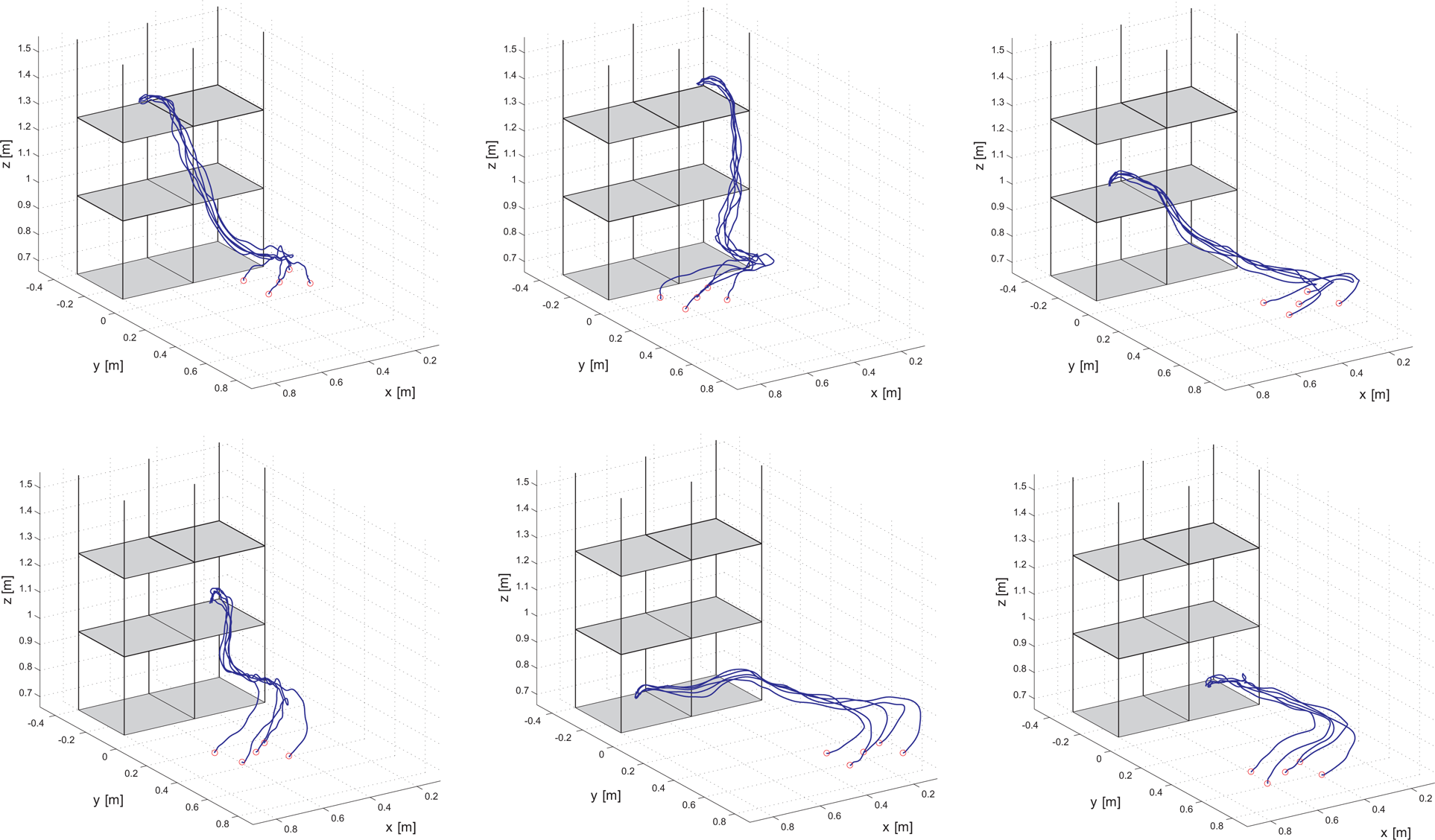
Newly generated trajectories. The goal areas i. e. the shelving units, are shown in black and gray. The new trajectories are shown in blue, while its starting points are marked with red circles. Each series now covers all of the starting area for each goal area.

The demonstrated trajectories were obtained by kinaesthetically guiding the robot arm, as seen in Fig. 7. For each of the six goal areas, we captured a series of five movements that roughly covered one-sixth of the starting area − 30 movements altogether. These captured movements are shown in Fig. 8. For each movement, the object's starting position was estimated by stereo vision and saved together with the trajectory data. With the selected k -means clustering algorithm, we constructed the database using the 30 example trajectories. The hierarchical database included transition graphs at different levels of granularity, as explained in Section 2. The resulting database consisted of 20 levels with 4,133 nodes at the deepest level.

5.4 New example series

The goal of the next step was to discover six new series of reaching movements, one for each shelf. In contrast to the training trajectory data, which covered only one-sixth of the starting zone for each shelving unit - the newly discovered series covered the entire starting zone. Each new series consisted of 30 movements, which were associated with the input parameters x _st^k, while x _end^k were all equal to the unique end position associated with the corresponding shelving unit. In the interest of greater precision, we generated new trajectories at the deepest level in the database; therefore, the majority of the new movements could not be generated through the transition graph search alone. We used a hierarchical search to discover partial paths and combined them through DMP-based interpolation, as described in Section 3. When interpolating a sequences of partial paths with DMPs, we reduced the number of basis functions at break the nodes in order so as to further smoothen the transition. An example interpolated movement, generated from partial paths, can be seen in Fig. 9. We constructed six new series of trajectories from a database consisting of six smaller series. In this way, we expanded 30 demonstrated reaching movements to 180 new reaching movements, each of them retaining the shape of the movement and the precision needed for the task. Although the computational time for synthesizing each new movement was on average around 12 s, it should be noted that this was achieved using non-optimized MATLAB code and could be reduced drastically by implementing optimized code in a faster programming language, e.g., C++. The new sets of movements consisted of movements from the entire starting area to every shelving unit, and can be seen in Fig. 10.

5.5 Statistical generalization

Although the example trajectories now cover the entire starting zone, it is highly unlikely that the object would be located precisely at one of the 30 starting positions. Because of this, we use statistical methods to generalize newly found trajectories and compute a movement for every starting position of our object. Some example trajectories obtained by the statistical generalization of one of the new series of trajectories can be seen in Fig. 11 and Fig. 12.

Figure 11.

New trajectories obtained by statistical generalization. Trajectories used for generalization are in black, whereas the synthesized trajectories are shown as red dashed lines. Starting points are marked with circles. The newly generated trajectories are adapted to the new starting positions.

Figure 12.

New trajectories obtained by statistical generalization. Trajectories used for generalization are in black, whereas the synthesized trajectories are shown as red dashed lines. Note that the generalized trajectories are similar to the original ones.

With the generalization of newly found series of shelf-placing movements, our robot was able to pick the object from any position in the starting area and place it at any of the six goal positions on the shelving unit with a smooth motion while avoiding collisions with the shelf, as can be seen in video (http://tinyurl.com/VideoAppendix-HDb). One of these new placing movements can also be seen in Fig. 13. All the movements avoid collision with the shelf because the demonstrated trajectories avoid such collisions. This property is preserved by the graph search, the hierarchical search and the statistical generalization, which result in trajectories that are similar to the parts of the demonstrated trajectories.

Figure 13.

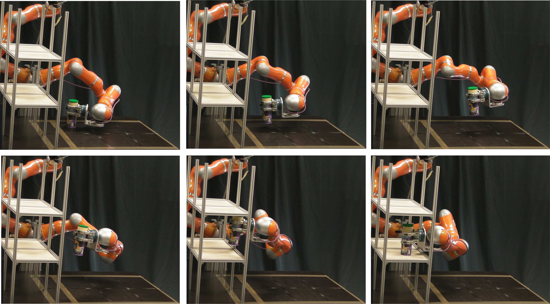
Execution of a new movement. The movement with such a combination of start and goal position was not contained in the training data. Even if the object is positioned at a random spot inside the starting area, the robot can successfully place it to any of the 6 desired shelving unit parts.

5.6 Synthesis in the joint space

The main experiment synthesized new movement primitives using data in Cartesian space (2). This means that clustering, a partial path search, DMP interpolation and statistical generalization were done in Cartesian space. This subsection of the evaluation focuses on synthesizing new primitives from data in the robot's joint space instead. The same human demonstrations for the same pick-and-place task were used. However, while the approach for synthesizing new primitives remained the same, the state vectors were now defined in the robot's joint space (3). Once the sample motion data was built, a hierarchical database with transition graphs was constructed. The database consisted of 21 levels with 3,464 nodes at the deepest level. The proposed approach managed to find all the new trajectories using this database, i.e., the same number of trajectories as in the main experiment, connecting all the start positions with all the racks. A comparison of an example new trajectory synthesized using Cartesian space data with a trajectory synthesized with the joint space data is shown in

Figs. 14 and 15. While some discrepancies can be noted between the majority of the new trajectories, the new trajectories retain the needed shape to execute a given task.

Figure 14.

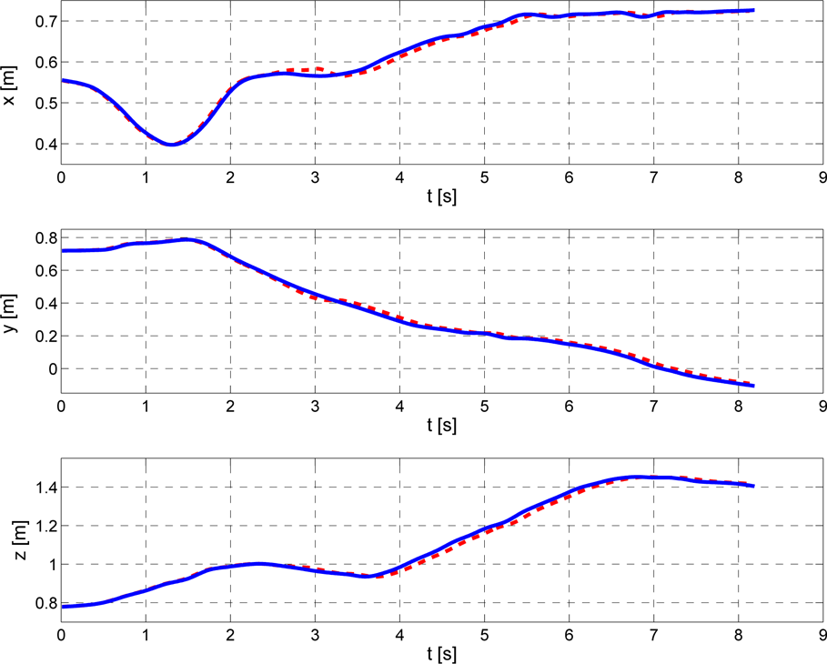
An example of a newly generated trajectory synthesized using joint space data for each of the three dimensions. The figure shows two trajectories. A new trajectory generated using joint space data and then transformed to Cartesian space is denoted with a dashed red line, while a trajectory gained in the previous experiment, using Cartesian space data, is denoted with a blue line. While the trajectories are mainly identical, there are some minor discrepancies.

Figure 15.

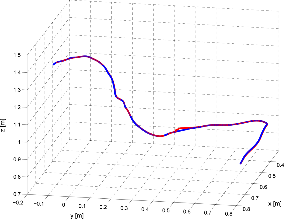
An example of a newly generated trajectory synthesized using joint space data in 3 dimensions. The figure shows two trajectories. A new trajectory generated using joint space data and then transformed to Cartesian space is denoted with a red line, while a trajectory gained in the previous experiment, using Cartesian space data, is denoted with a blue line. While the trajectories are mainly identical, there are some minor discrepancies.

6. Discussion

The experimental results showed that it is possible to discover new movement primitives in a database of example demonstrated movements. Unlike many other approaches in imitation learning, it is assumed that the training database consists of different types of movements. They are combined by exploiting the interconnections between the movements using graph search technologies. This search process generates new movements that are not part of the initial training database. A novel hierarchical graph search procedure was developed, which starts at the highest level where the direct connection between the desired start and end robot configurations exists, and progresses through the transition graph levels, finally producing a series of partial paths connecting the two nodes at the desired level of granularity. These partial paths are combined using DMP-based interpolation. The interpolation procedure ensures that the newly generated trajectories are smooth. In this way, connections are generated between desired configurations, even if they do not belong to the same example component at the desired level of granularity. The proposed approach reduces the burden of demonstrating many trajectories while preserving the needed precision, shape and smoothness of movement. This was shown by evaluating the hierarchical search, where 30 demonstrated reaching movements were expanded to 180 new reaching movements, each of them retaining the shape of movement and precision needed for successfully executing the task. While this task could be accomplished by motion planning algorithms, we believe that it shows the applicability of our approach by extensively expanding the initial database through a combination of different parts of movements, and thus reducing the burden of multiple demonstrations usually needed for programming by demonstration. By merging the results of the hierarchical search with statistical generalization, a complete representation of a new movement primitive could be constructed.

In our evaluation, the data are acquired through kinaesthetic guidance by a human demonstrating a pick-and-place task. As the task is defined in Cartesian space, the human will automatically devote more attention to the robot's end-effector in Cartesian space than to the pose of the robot. This is one of the reasons Cartesian space data was used throughout the main experiment. In order to show the robustness of the proposed approach, an additional experiment using joint space data from the same demonstrations was performed. While no extra attention was paid to the robot's pose during the kinaesthetic guidance, the joint trajectories still shared sufficiently similar parts so as to make synthesis and interpolation viable.

While the prosed approach for the synthesis of new movement primitives is related to the work of Yamane et al. [27], some fundamental disparities need to be noted. While they proposed clustering the state vectors from the example trajectories using principal component analysis (PCA) and a minimum-error thresholding technique [11], this paper evaluates various clustering approaches and proposes clustering the data with the k -means algorithm [16], as it is shown to be more efficient. Note that, unlike Yamane et al., whose interest was primarily in full-body movements, this paper focus on arm trajectories and manipulation tasks, which often require finer precision. The criterion for stopping further clustering is therefore based on the variability of the data in clusters rather than solely on the number of nodes, which enables higher precision. It mainly needs to be emphasized that, in contrast to Yamane et al., we do not assume connections between the desired start and end nodes at the desired level. Instead, a novel approach of a hierarchical database search is used to find optimal partial paths.

Future work will involve the evaluation of our approach on larger databases consisting of more diverse movements. With the increasing size of the database, we might encounter greater computational costs, but the research performed by the computer animation community has shown that such databases can be processed in a reasonable time. The implementation of an optimized code in a faster programming language would also reduce computational times. The database could also be expanded with additional data, e.g., information about objects involved in the action. It could be extended to generate human-robot cooperative movements [28]. Forces and torques arising during manipulation actions could also be encoded in the database and used for compliant movement generation.

Footnotes

Multimedia Appendix

http://tinyurl.com/VideoAppendix-HDb

8.

The research leading to these results has received funding from the European Community's Seventh Framework Programme FP7/2007-2013 (Specific Programme Cooperation, Theme 3, Information and Communication Technologies) under grant agreement no. 270273, Xperience.

References

Breazeal

Cynthia

and Scassellati

Brian

. Robots that imitate humans. Trends in cognitive sciences, 6(11):481–487, 2002.

Calinon

Sylvain

D'halluin

Florent

Sauser

Eric L

Caldwell

Darwin G

, and Billard

Aude G

. Learning and reproduction of gestures by imitation. Robotics & Automation Magazine, IEEE, 17(2):44–54, 2010.

Davies

David L

and Bouldin

Donald W

. A cluster separation measure. Pattern Analysis and Machine Intelligence, IEEE Transactions on, (2):224–227, 1979.

Dillmann

Rüdiger

. Teaching and learning of robot tasks via observation of human performance. Robotics and Autonomous Systems, 47(2):109–116, 2004.

Dun

. A fuzzy relative of the isodata process and its use in detecting compact well-sparated cluster. J Cybern, 3:32–57, 1973.

Forte

Denis

Gams

Andrej

Morimoto

Jun

, and Ude

Ales

. On-line motion synthesis and adaptation using a trajectory database. Robotics and Autonomous Systems, 60(10):1327–1339, 2012.

Hersch

Micha

Guenter

Florent

Calinon

Sylvain

, and Billard

Aude

. Dynamical system modulation for robot learning via kinesthetic demonstrations. Robotics, IEEE Transactions on, 24(6):1463–1467, 2008.

Ijspeert

Auke Jan

Nakanishi

Jun

Hoffmann

Heiko

Pastor

Peter

, and Schaal

Stefan

. Dynamical movement primitives: learning attractor models for motor behaviors. Neural computation, 25(2):328–373, 2013.

Inamura

Tetsunari

Toshima

Iwaki

Tanie

Hiroaki

, and Nakamura

Yoshihiko

. Embodied symbol emergence based on mimesis theory. The International Journal of Robotics Research, 23(4–5):363–377, 2004.

10.

Khansari-Zadeh

S Mohammad

and Billard

Aude

. Learning stable nonlinear dynamical systems with gaussian mixture models. Robotics, IEEE Transactions on, 27(5):943–957, 2011.

11.

Kittler

Josef

and Illingworth

John

. Minimum error thresholding. Pattern recognition, 19(1):41–47, 1986.

12.

Kober

Jens

Wilhelm

Andreas

Oztop

Erhan

, and Peters

Jan

. Reinforcement learning to adjust parametrized motor primitives to new situations. Autonomous Robots, 33(4):361–379, 2012.

13.

Kovar

Lucas

Gleicher

Michael

, and Pighin

Frédéric

. Motion graphs. In ACM transactions on graphics (TOG), volume 21, pages 473–482. ACM, 2002.

14.

Kulić

Dana

Takano

Wataru

, and Nakamura

Yoshihiko

. Incremental learning, clustering and hierarchy formation of whole body motion patterns using adaptive hidden markov chains. The International Journal of Robotics Research, 27(7):761–784, 2008.

15.

Kulic

Dana

Takano

Wataru

, and Nakamura

Yoshihiko

. Online segmentation and clustering from continuous observation of whole body motions. Robotics, IEEE Transactions on, 25(5):1158–1166, 2009.

16.

MacQueen

James

Some methods for classification and analysis of multivariate observations. In Proceedings of the fifth Berkeley symposium on mathematical statistics and probability, volume 1, pages 281–297. Oakland, CA, USA., 1967.

17.

McLachlan

Geoffrey

and Krishnan

Thriyambakam

. The EM algorithm and extensions, volume 382. John Wiley & Sons, 2007.

18.

Moeslund

Thomas B

Hilton

Adrian

, and Krüger

Volker

. A survey of advances in vision-based human motion capture and analysis. Computer vision and image understanding, 104(2):90–126, 2006.

19.

Nakaoka

Shin'ichiro

Nakazawa

Atsushi

Kanehiro

Fumio

Kaneko

Kenji

Morisawa

Mitsuharu

Hirukawa

Hirohisa

, and Ikeuchi

Katsushi

. Learning from observation paradigm: Leg task models for enabling a biped humanoid robot to imitate human dances. The International Journal of Robotics Research, 26(8):829–844, 2007.

20.

Pollard

Nancy S

Hodgins

Jessica K

Riley

Marcia J

, and Atkeson

Christopher G

. Adapting human motion for the control of a humanoid robot. In Robotics and Automation, 2002. Proceedings. ICRA'02. IEEE International Conference on, volume 2, pages 1390–1397. IEEE, 2002.

21.

Rose

Charles

Cohen

Michael F

, and Bodenheimer

Bobby

. Verbs and adverbs: Multidimensional motion interpolation. Computer Graphics and Applications, IEEE, 18(5):32–40, 1998.

22.

Safonova

Alla

and Hodgins

Jessica K

. Construction and optimal search of interpolated motion graphs. In ACM Transactions on Graphics (TOG), volume 26, page 106. ACM, 2007.

23.

Schaal

Stefan

. Is imitation learning the route to humanoid robots? Trends in cognitive sciences, 3(6): 233–242, 1999.

24.

Shotton

Jamie

Sharp

Toby

Kipman

Alex

Fitzgibbon

Andrew

Finocchio

Mark

Blake

Andrew

Cook

Mat

, and Moore

Richard

. Real-time human pose recognition in parts from single depth images. Communications of the ACM, 56(1):116–124, 2013.

25.

Sidenbladh

Hedvig

Black

Michael J

, and Sigal

Leonid

. Implicit probabilistic models of human motion for synthesis and tracking. In Computer Vision—ECCV 2002, pages 784–800. Springer, 2002.

26.

Ude

Aleš

Atkeson

Christopher G

, and Riley

Marcia

. Programming full-body movements for humanoid robots by observation. Robotics and autonomous systems, 47(2):93–108, 2004.

27.

Yamane

Katsu

Yamaguchi

Yoshifumi

, and Nakamura

Yoshihiko

. Human motion database with a binary tree and node transition graphs. Autonomous Robots, 30(1):87–98, 2011.

28.

Yamane

Keisaku

Revfi

Marcel

, and Asfour

Tamim

. Synthesizing object receiving motions of humanoid robots with human motion database. In Robotics and Automation (ICRA), 2013 IEEE International Conference on, pages 1629–1636. IEEE, 2013.

No. of example trajectories	6×5
No. of state vectors	25270
No. of levels	20
No. of nodes at the deepest level	4133

Synthesis of New Dynamic Movement Primitives Through Search in a Hierarchical Database of Example Movements

Abstract

Keywords

1. Introduction

2. Generation of a hierarchical database of example movements

5.2 Clustering algorithm evaluation

Table 1. Properties of the constructed database No. of example trajectories 6×5 No. of state vectors 25270 No. of levels 20 No. of nodes at the deepest level 4133

5.5 Statistical generalization

Footnotes

Multimedia Appendix

8.

References

Table 1.
Properties of the constructed database

No. of example trajectories 6×5

No. of state vectors 25270

No. of levels 20

No. of nodes at the deepest level 4133