Sage Journals: Discover world-class research

Abstract

The aim of this paper is to deploy a time-of-flight (ToF) based photonic mixer device (PMD) camera on an Autonomous Ground Vehicle (AGV) whose overall target is to traverse from one point to another in hazardous and hostile environments employing obstacle avoidance without human intervention. The hypothesized approach of applying a ToF Camera for an AGV is a suitable approach to autonomous robotics because, as the ToF camera can provide three-dimensional (3D) information at a low computational cost, it is utilized to extract information about obstacles after their calibration and ground testing and is mounted and integrated with the Pioneer mobile robot. The workspace is a two-dimensional (2D) world map which has been divided into a grid/cells, where the collision-free path defined by the graph search algorithm is a sequence of cells the AGV can traverse to reach the target. PMD depth data is used to populate traversable areas and obstacles by representing a grid/cells of suitable size. These camera data are converted into Cartesian coordinates for entry into a workspace grid map. A more optimal camera mounting angle is needed and adopted by analysing the camera's performance discrepancy, such as pixel detection, the detection rate and the maximum perceived distances, and infrared (IR) scattering with respect to the ground surface. This mounting angle is recommended to be half the vertical field-of-view (FoV) of the PMD camera. A series of still and moving tests are conducted on the AGV to verify correct sensor operations, which show that the postulated application of the ToF camera in the AGV is not straightforward. Later, to stabilize the moving PMD camera and to detect obstacles, a tracking feature detection algorithm and the scene flow technique are implemented to perform a real-time experiment.

Keywords

3D ToF Camera PMD Camera Pioneer Mobile Robots Path-planning

1. Introduction

As an AGV must be able to adequately sense its surroundings in order to operate in unknown environments and execute autonomous tasks, vision sensors provide the necessary information required for it to perceive and avoid any obstacles to accomplish autonomous path-planning. Hence, the perception sensor becomes the key sensory device for perceiving the environment in intelligent mobile robots, and the perception objective depends on three basic system qualities, namely rapidity, compactness and robustness [1].

Over the last few decades, many different types of sensors [2] have been developed in the context of AGV path-planning to avoid obstacles [3] such as infrared sensors [4], ultrasonic sensors, sonar [5], LADAR [6], laser rangefinders [7], camera data fused with radar [8] and stereo cameras with a projector [9]. These sensors’ data along with data processing techniques are used to update the positions and directions of the vertices of obstacles. However, these sensor systems are unable to provide necessary information without ease about any surroundings.

As the world's attention is increasingly focusing on automation in every field, extracting 3D information about an obstacle has become a topical and challenging task. As such, an appropriate sensor is required to obtain 3D information that has small dimensions, low power consumption and real-time performance. The main limitation of a 2D camera is that, as it is the projection of 3D information onto a 2D image plane, it cannot provide complete information of the entire scene. Thus, the processing of these images will depend upon the view point (rather than the actual information about the object). In order to overcome this drawback, the use of 3D information has emerged. In general, researchers use a setup consisting of a charge-coupled device (CCD) camera and light projector in order to obtain a 3D image, such as that of the 3D visualization of rock [9].

A 3D sensor is selected for our work, which is based on the photonic mixer device (PMD) technology that delivers range and intensity data with low computational cost as well as compactness and economical design with a high frame rate. This camera system delivers absolute geometrical dimensions of obstacles without depending upon the object surface, distance, rotation or illumination. Hence, it is rotation-, translation- and illumination-invariant [10]. Nowadays, RGBD cameras (e.g., Kinect, Asus Xtion, Carmine) have been widely used in object recognition and mobile robotics applications. However, these RGBD cameras cannot operate in outdoor environments [11]. A PMD camera with a working range of (0.2 – 7 metres) provides better depth precision compared to Kinect (0.7 – 3.5 metres) and Carmine (0.35 – 1.4 metres).

However, the PMD camera is constrained by its limited FoV, namely its need to adjust the camera mounting downwards to obtain a greater view of the ground. The specific angle of this mounting is explained in this paper; nonetheless, it was unexpected that light incident at different angles to the ground would result in significant receiver loss and distortion of distance measurements due to scattering. The camera is mounted on the front of the robot through brackets that enable variable camera mounting angles at a static angle of tilt - it is perceived that this configuration would enable the best compromise between the ground conception and a straight ahead conception as a function of the camera tilt angle Ψ. Due to being mounted above the robot, it would be necessary to flag closer obstacles so as to reduce the blind spot in front of the robot. Because of these considerations, a more optimal camera angle is adopted. To ensure that the top-most pixels are observed directly ahead of the robot, thereby giving an adequate conception of obstacles and maximizing the ground plane conception, various analyses of the camera performance are carried out in this paper.

Later, the parametric calibration for the PMD cameras is performed by obtaining necessary camera parameters to derive the true information of the imaging scene. The imaging technology of the PMD camera is better understood whereby camera pixels provide a complete image of the scene with each pixel detecting the range data stored in a 2D array, which are utilized and interpreted in this paper to extract information about the surroundings. A few experiments are carried to measure the camera's parameters and distance errors with respect to each pixel.

To determine the difference between the function of the camera in an environment similar to that claimed by the manufacturer data sheet, white surface testing and grass surface testing are conducted for the PMD camera. This also provided a means to compare the performance of the camera from a flat white surface to a flat grassy surface. Later, the camera data is synchronized with the instantaneous orientation and position of the platform (and thus the camera), which translates the Cartesian coordinates into squares of grids. It reconstructed the ground region (extremities that the camera could see) into a grid of suitable grid cells which are imputed to the path-planning algorithm.

During real-time experimentation, the grid-based Efficient D^∗ Lite path-planning algorithm and scene-flow technique were programmed on the Pioneer onboard computers using the OpenCV and OpenGL libraries. In order to compensate for the ego-motion of the PMD camera, which is aligned with the AGV coordinates, a features detection algorithm using Good – Features – to – Track from the OpenCV library is adopted.

The paper is organized as follows: a brief comparison of the 3D sensors and their fundamental principles is presented in Section II. In Section III, the calibration of the PMD camera is performed by parametric calibration. Section IV presents the manipulation of the PMD camera data. In Section V, several standardized tests are devised to characterize the PMD camera and Section VI describes the experimental results.

2. ToF-based 3D Cameras - state-of-the-art

Nowadays, 3D data are required in the automation industries for analysing the visible space/environment. The rapid acquisition of 3D data by a robotic system for navigation and control applications is required. New 3D cameras at affordable prices which have been successfully developed using the ToF principle to resemble LIDAR scanners. In a ToF camera unit, a modulated light pulse is transmitted by the illumination source and the target distance is measured from the time taken by the pulse to reflect from the target back to the receiving unit. PMD technologies have developed 3D sensors using the ToF principle, which provide for a wide range of field applications with high integration and cost-effective production [12].

ToF cameras do not suffer from missing texture in the scene or bad lighting conditions, are computationally less expensive than stereo vision systems and - compared with laser scanners - have higher frame rates and more compact sensors, advantages which make them ideally suited for 3D perception and motion reconstruction [13]. The following advantages of ToF cameras are found in the literature:

Simplicity: compared with 3D vision systems, a ToF-based system is very simple and compact, consisted no moving parts and having built-in illumination adjacent to its lens.

Efficiency: only a small amount of processing power is required to extract distance information using a ToF camera.

Speed: in contrast to laser scanners that move and measure point-by-point, ToF cameras measure a complete scene with one shot at up to 100 frames-per-second (fps), much faster than their laser alternatives.

In addition, ToF cameras have been applied in robotic applications for obstacle avoidance [14, 15]. There are many other applications in various fields [16] that have gained substantial research interest following the advent of the range sensor, such as robotic and machine vision in the field of mobile robotics search and rescue [17, 18], path-planning for manipulators [19], the acquisition of 3D scene geometry [20], 3D sensing for automated vehicle guidance and safety systems, wheelchair assistance [21], outdoor surveillance [22], simultaneous localization and mapping (SLAM) [23], map building [24], medical respiratory motion detection [25], robot navigation [26], semantic scene analysis [27], mixed/augmented reality [28], gesture recognition [29], markerless human motion tracking [30], human body tracking and activity recognition [31], 3D reconstruction [32], domestic cleaning tasks [33] and human-machine interaction [34, 35].

The authors in [36] used stereo cameras to identify the 3D orientation of the object and ToF cameras have been used for 3D object scanning, employing different approaches, such as passive image-based and super-resolution methods with probabilistic scan alignment [37]. The 3D range camera obtains range data and locates the positions of objects in its FoV [38], while active sensing technologies have been used as an active safety system for construction applications and accident avoidance [39].

The ToF camera has been used to detect the standard size of obstacles and it can be used for obstacle and travel path detection applications for the blind and visually impaired by combining 3D range data with stereo audio feedback [21], using the algorithm to segment obstacles according to intensity and the 3D structure of the range data. Gesture recognition has been performed based on shape contexts and simple binary matching [40] whereby motion information is extracted by matching the difference in the range data of different image frames. The measurement of shapes and deformations of metal objects and structures using ToF range information and heterodyne imaging are discussed in [41].

2.1 The Basic ToF Principle

A single pixel consists of a photo-sensitive element (e.g., a photo diode) which converts incoming light into current. The distance between the camera and an object is determined by the ToF principle and the time taken by the light to travel from the illumination unit to the receiver is directly proportional to the distance travelled by the light [42], with the delay time t_D given by

t_{D} = 2 \times \frac{D_{o b j}}{c_{o}}

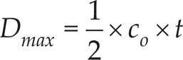
where D_obj is the object distance in metres and c_o is the velocity of light in m/s.

The pulse width of the illumination determines the maximum range that the camera can handle, which can be determined by

D_{m a x} = \frac{1}{2} \times c_{o} \times t

The distance between the sensor and the object is half the total distance travelled by the radiation. The two different distance measurement methods described by T. Kahlmann et al. [42]) are the pulse run time and the phase shift determination.

In the ToF camera, the distance between the camera and the obstacle is calculated by the autocorrelation function of the electrical and optical signals, which is analysed by a phase-shift algorithm (Figure 1). Using four samples, A1, A2, A3 and A4 (each shifted by 90 degrees), the phases of the received signals - which are proportional to the distance - can be calculated using the following equation[43].

The phase shift, φ, is

φ = a r c t a n (\frac{A_{1} - A_{3}}{A_{2} - A_{4}})

(1)

In addition to the phase shift of the signal, a_r, the signal strength of the received signal (amplitude) and b_r offsets from the samples which represent the greyscale value of each pixel can be determined by

a_{r} = \frac{\sqrt{{(A_{1} - A_{3})}^{2} - {(A_{2} - A_{4})}^{2}}}{2}

(2)

b_{r} = \frac{A_{1} + A_{2} + A_{3} + A_{4}}{4}

(3)

The depth data is calculated from the phase information φ as

d_{r} = \frac{c_{o}}{2 f_{m o d}} \times \frac{φ}{2 π}

(4)

where f_mod is the modulation frequency and c_o is the speed of light.

Figure 1.

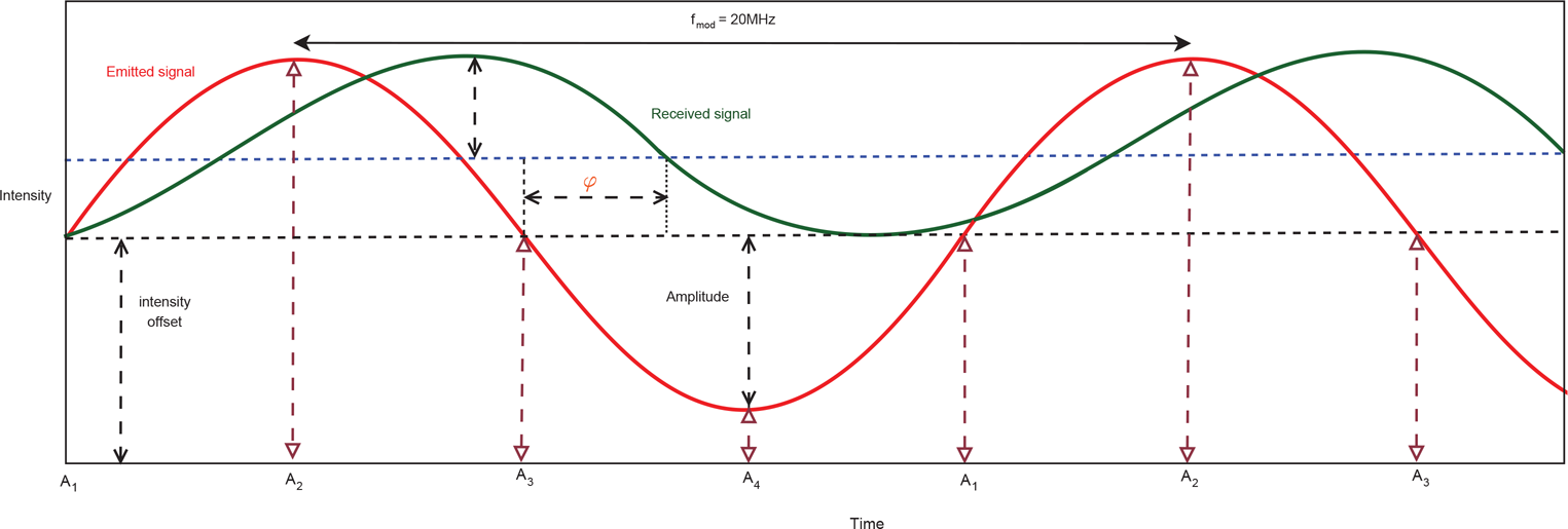
Phase shift distance measurement principle: optical sinusoidally modulated input signal, sampled with four sampling points per modulation period [11]

The PMD CamCube 2.0 and PMD S3 cameras are shown in Figures 2 and 3 and their specifications are listed in Tables 1 and 2.

Figure 2.

PMD[vision] CamCube 2.0 camera

Figure 3.

PMD[vision] S3 Camera

Table 1.

PMD CamCube 2.0 specification

Integration time	200 ms
Modulation frequency	23 MHz
Wavelength	13 m
Pixel resolution	200[H]x200[V]
FoV V/H []	40/40
Internal illumination[nm]	870

Table 2.

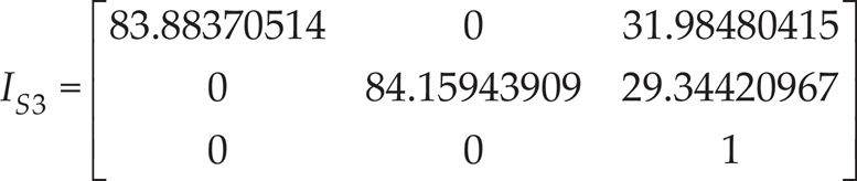
PMD[vision]S3 specification

Integration Time	200 ms
Modulation frequency	23 MHz
Pixel resolution	48[H]x64[V]
FoV H/V []	40/30
Internal illumination[nm]	850

3. Parametric Calibration

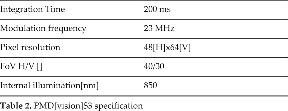
The PMD CamCube 2.0 and PMD S3 cameras, developed by PMD Technologies Inc. and which are based on the ToF principle, are used. The PMD CamCube 2.0 camera's receiver optics has 200 by 200 pixels with an FoV of 40(H)/40(V) degrees. The PMD S3 has an FoV of 40(H)/30(V) degrees with 64 HP and 48 VP, and thus in total is able to return 3,072 distance measurements in a square array.

In this section, the calibration of the PMD cameras is performed by a parametric calibration procedure that provides necessary camera parameters. These parameters can be used to derive the true information of the imaging scene. The procedure can also provide the translational vector and rotational matrix on the 3D space for the camera which can be used to find the true information about the coordinate positions of the camera and the imaging scenario.

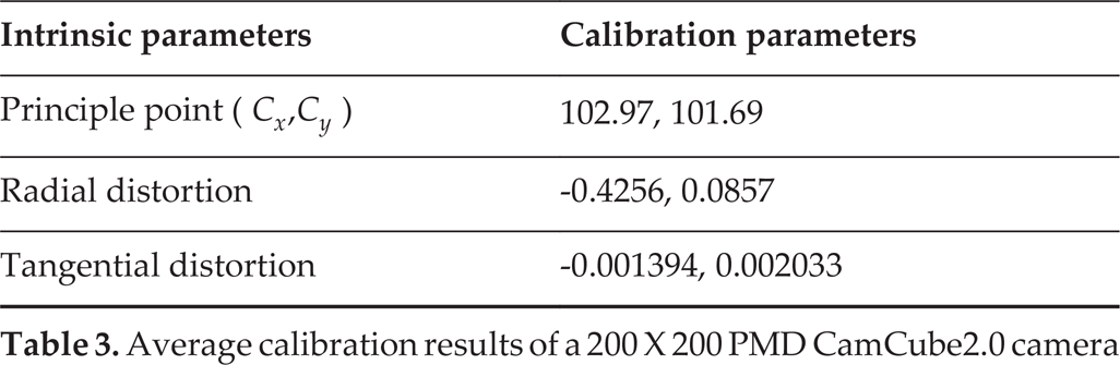
Basically, the intrinsic parameters of the camera provide the transformation between the image coordinates and the pixel coordinates of the camera [44, 45]. The intrinsic matrix is given by

[\begin{matrix} f_{c a m} / S_{x} & 0 & C_{x} \\ 0 & f_{c a m} / S_{y} & C_{y} \\ 0 & 0 & 1 \end{matrix}]

(5)

where f_cam is the focal length of the camera, S_x and S_y are the pixel sizes of the camera in the x and y axes respectively, and C_x and C_y are the principal points of the sensor array. To obtain the camera parameters, an experimental setup is developed in which the calibration process of the PMD CamCube 2.0 and PMD S3 camera is performed by capturing intensity and depth images of the chequerboard with different orientations, as shown in Figures 4 and 5. The chequerboard has black and white squares of known dimensions, each printed on a 21 cm × 29.7 cm A4 paper. The ‘OpenCV'¹, and is used to estimate the intrinsic parameters as well as the radial distortion in a Debian 6.0 installed laptop.

Figure 4.

Parametric calibration (corners: x=9, y=6; spacing x=y=27 mm)

The calibration test is also conducted with three different chequerboard squares of dimensions (9 × 6), (5 × 7) and (6 × 4) and corner spacing of 27 mm, 40 mm, 100 mm, respectively. The manufacturer's values for the PMD CamCube 2.0 camera are:

pixel size, S_x = S_y = 45 μm,

Aspect ratio = 1, Skew =0,

focal length, f_cam = 12.8 mm and

The manufacturer's value for the PMD S3 camera are:

pixel size, S_x = S_y = 100 μm,

Aspect ratio = 1.333, Skew =0,

focal length, f_cam = 8.4 mm and

Figure 5.

Parametric calibration (corners: x=5, y=7; spacing x=y=40 mm)

The main parameters of the intrinsic matrix are the focal length, the principal point, the skew coefficient and distortions. It defines the optical, geometric and digital characteristics of the camera which are calculated using Equations 6 and 7.

I_{c u b e 2.0} = [\begin{matrix} 2.8951 e^{2} & 0 & 1.0297 e^{2} \\ 0 & 2.89268 e^{2} & 1.016920 e^{2} \\ 0 & 0 & 1 \end{matrix}]

(6)

I_{S 3} = [\begin{matrix} 83.88370514 & 0 & 31.98480415 \\ 0 & 84.15943909 & 29.34420967 \\ 0 & 0 & 1 \end{matrix}]

(7)

The distortion is caused mainly by the camera optics and is directly proportional to its focal length. The radial distortion and tangential distortion are the lens distortion effects introduced by real lenses. Generally, there are four distortion parameters, i.e., two radial and two tangential distortion coefficients, which are calculated as:

D i s t o r t i o n_{c u b e 2.0} = [\begin{matrix} - 0.4256 & 0.8573 e^{- 01} & - 1.3939 e^{- 03} & 2.0328 e^{- 03} \end{matrix}]

(8)

D i s t o r t i o n_{s 3} = [\begin{matrix} - 0.4394 & 1.0112 & 4.4002 e^{- 03} & - 7.8725 e^{- 05} \end{matrix}]

(9)

Table 3.

Average calibration results of a 200 × 200 PMD CamCube2.0 camera

Intrinsic parameters	Calibration parameters
Principle point (C_x, C_y)	102.97, 101.69
Radial distortion	−0.4256, 0.0857
Tangential distortion	−0.001394, 0.002033

Table 4.

Average calibration results of a PMD S3 camera

Intrinsic parameters	Calibration parameters
Radial distortion	−0.4394, 1.0112
Tangential distortion	−0.0044002, −7.8725e^−0.5

By calibrating the camera, intrinsic and extrinsic camera parameters are detected to eliminate the geometric distortion of the images.

Thus, the transformation between a point in the scene/world coordinates system P_wor and the image plane coordinate system O_cam is provided through a rotational matrix R_ext and a translational vector T_ext. The joint rotation-translation matrix [R_ext | T_ext] determines the extrinsic parameters of the camera.

Rotation matrix:

R_{e x t} = [\begin{matrix} - 0.437390661 & 1.0 & 0.0 & 0.0 \\ - 4.42766333 & 0.0 & 1.0 & 0.0 \\ 0.35243243 & 0.0 & 0.0 & 1.0 \end{matrix}]

(10)

Translation vector:

T_{e x t} = [\begin{matrix} 1.0 & 0.0 & 0.0 & 7.7065 e^{- 0.3} \\ 0.0 & 1.0 & 0.0 & - 0.04777 \\ 0.0 & 0.0 & 1.0 & 0.0074 \\ 0.0 & 0.0 & 0.0 & 1.0 \end{matrix}]

(11)

[\begin{matrix} x_{c a m} \\ y_{c a m} \\ z_{c a m} \end{matrix}] = [\begin{matrix} R_{e x t} | T_{e x t} \end{matrix}] [\begin{matrix} x_{w o} \\ y_{w o} \\ z_{w o} \\ 1 \end{matrix}]

(12)

The relationship between the scene/world point P_wo and its projection p_cam can be written as

P_{c a m} = I_{c a m} [R_{e x t} | T_{e x t}] P_{w o}

(13)

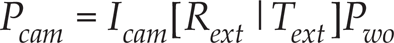
where (x_wo, y_wo, z_wo) are the coordinates of a point P_wo in the scene/world coordinate system and (x_cam, y_cam, z_cam) are the coordinates in the camera coordinate system.

4. Manipulation of PMD Camera Data

The camera's pixels provide a complete image of the scene, with each pixel detecting the intensity or projection of the optical image, respectively, while the range data obtained from each pixel is stored in a 2D array. The camera also provides the signal strength of the illumination and intensity information, which can be used to determine the quality of the distance value (a low amplitude indicates the low accuracy of the measured distance in a pixel). The coordinates of the object with respect to the PMD camera are obtained as a 2D matrix, with each element corresponding to a pixel. As the dimensions of the image frame depend upon its distance from the camera and the camera's field of view, an object's height and width can be calculated using its pixel elements [47].

Two different range frames of a rectangular object, i.e., X_d − near and X_d − far from the camera, are represented pictorially in Figure 6. The pixel-size projected on the object is different for the two frames and decreases as the distance between the camera and image frame increases since the object's area projected on the near frame (i_{x
_n} × i_{y
_n}) is different from that (i_{x
_f} × i_{x
_f}) on the far frame. As can be seen, except for the projected pixel size of each pixel, all the other parameters (Equations (14)–(19)) increase with an increase in the distance of the object frame from the camera.

Figure 6.

PMD camera's FoV and image frames

Using geometry;

l = t a n (F o V (H)) \times X_{d}

(14)

h = t a n (F o V (V)) \times X_{d}

(15)

P_{h} = \frac{l}{No.of pixels (H)}

(16)

P_{v} = \frac{h}{No.of pixels (V)}

(17)

i_{y} = P_{h} \times O_{v}

(18)

i_{x} = P_{v} \times O_{h}

(19)

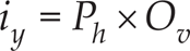
where l is the length of the image frame, h is the height of the image frame, X_d is the distance between the image frame and the camera, P_h is the projected pixel size of each pixel in the object along the horizontal axis, P_v is the projected pixel size of each pixel in the object along the vertical axis, O_h is the number of object-occupied pixels along the horizontal axis in the image frame, O_v is the number of object-occupied pixels along the vertical axis in the image frame, i_x is the total length of the object in the image frame, and i_y is the total height of the object in the image frame.

To obtain accurate readings, an experimental setup is made as shown in Figure 7(a). The camera and test object are placed on a horizontal rail, as shown in Figure 7, and the test object is moved to different distances without altering the position of the camera. A rectangular box of known dimensions (157 mm (length) × 80 mm (height)) is used as the reference object and its lengths and heights at different distances calculated using the readings from the camera, as previously discussed and illustrated in Figure 8, which are compared with the actual dimensions and the relative error, are calculated. Relative accuracies with respect to distance are shown in Figure 9, with the calculated lengths and heights of the test object plotted as blue and green lines, respectively. It can be seen that the relative error is less than ±3%.

Figure 7.

Experimental setup for calibration

Figure 8.

Experiment 1: rectangular box placed at different distances

Figure 9.

Plots of distance vs relative error

4.1 Camera Mounting Angle

The 3D model of the Pioneer 3DX with the cameras mounted at a tilt angle of Ψ =0 is created in Google Sketch-Up, and the dimensions of the AGV and the camera's FoV extended to 7,000 mm are drawn to closely resemble the actual situation in order to assist the perception of the work (Figure 10).

Figure 10.

3D model depicting P3DX AGV

As can be seen, for a camera orientation of Ψ = 0, a large number of captured data would not be necessary to flag obstacles (due to being above the robot), and the blind spot in front of the robot could ideally be reduced. Because of these considerations, a more optimal camera angle was adopted - this angle was determined as half the vertical FoV of the PMD.

ψ = 0.5 \times F o V

(20)

Setting Ψ ensured that the top-most pixels were observed directly ahead of the robot, thereby providing an adequate detection of obstacles while maximizing the ground plane conception. The sketch shown below illustrates the mounting concept, the grid (localized) and the cameras’ FoV projected as understood.

Figure 11.

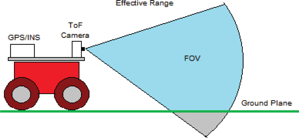
Sketch of the configuration with FoV

Figure 12.

Interpretation of PMD camera data into the occupancy grid

Following the creation of the 3D model to depict the developmental robot and its FoV, the MATLAB trigonometry toolbox for spherical co-ordinates was engaged to determine the specific placement of the ToF cameras’ data points. The distance measurements returned per pixel could be thought of as individual measurements at a known elevation and azimuth, and thus could be projected to intersect the ground plane if they are within the maximum range.

The ToF camera data are converted into Cartesian coordinates for the grid mapping using the following transformation,

x = r \times c o s (θ - ψ) \times c o s γ

(21)

y = r \times c o s (θ - ψ) \times s i n γ

(22)

z = [r \times s i n (θ - ψ) + h]

(23)

where x is the distance in front of the AGV [mm], y is the distance left of the AGV's midpoint [mm], z is the height above the AGV's ground level [mm], θ is the elevation from the camera midpoint [degrees], γ is the azimuth from the camera midpoint [degrees], Ψ is the downwards camera tilt [degrees] and h is the camera height above the ground from the centre of the receiver [mm].

Figure 13.

Pictorial representation of the co-ordinates

The following figures produced in MATLAB illustrate the projection of the individual pixels for a mounting angle of −15 degrees. The points on the plots show the projected position of the pixels in 3D space prior to the ground plane being considered and after it has been used as a boundary. The blue pixels show pixels that are above 0 degrees and the green pixels reflect the pixels that are below or on the ground plane.

Figure 14.

Non-truncated by the ground plane (−15 degrees)

Figure 15.

Truncated by the ground plane (−15 degrees)

5. Experimentation and Analysis

A PMD CamCube 2.0 camera is mounted on the Pioneer 3DX mobile robot as depicted in Figure 16, whereas the PMD S3 camera is hinged on the Pioneer AT robot. These PMD cameras provide Cartesian coordinates expressed in metres, with a correction which compensates for the radial distortions of the optics [48]. The coordinate system is right-handed, with the Z_cam coordinate increasing along the optical axis away from the camera, the Y_cam coordinate increasing vertically upwards and the X_cam coordinate increasing horizontally to the left - all from the point of view of the camera (or someone standing behind it). The origin of the coordinate system (0, 0, 0) is at the intersection of the optical axis and the front of the camera. As the cameras are statically fixed on top of the AGV's at a static angle of tilt of Ψ, their coordinates are aligned with those of the AGV's which provide the +12V power to run the camera.

Figure 16.

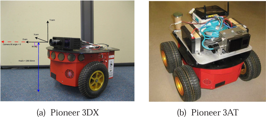
PMD mounted on the Pioneer robots

For these two mobile robots, the camera heights h were measured from the centre of the camera receiver to a level ground plane as h_S3onP3AT = 347.9 mm and h_{CamcubeonP3DX} = 286.50 mm.

In this section, several standardized tests are devised to characterize the PMD camera. The code that is written comprehensively analyses the camera mounting angle sweep tests when the AGV is stationary. Code has not been written to handle the reading of the moving tests with and without objects; however, results for these scenarios were used by applying the raw functionality of the program. This section intends to explain in-depth how to conduct the still angle sweep tests as well as how the moving tests and object recognition tests were performed.

To obtain a greater view of the ground, and necessarily, the camera mounting angle pointing downwards was adjusted. The specific angle of this mounting is explained; nonetheless, it was unexpected that the IR light incident on the angles to the ground plain would result in significant receiver loss and distortion of the distance measurements.

5.1 Stationary Angle Sweeps

To perform this type of testing, the PMD camera was mounted at a constant height such that the angle subtended by the camera's FoV to the ground could be varied. The ground plane is also flat and uniform (a flat grass field fits this criteria). This concept is illustrated in the figures below - in these figures, the camera is mounted on the AGV and a hinge-type bracket enables the mounting angle to be changed.

Figure 17.

Sweep of mounting angles

In addition, a white surface was recreated using plain white paper and a sweep of the camera angles was conducted. Testing the camera on a white surface recreated the conditions outlined by the PMD S3 data sheet, whereby the white, grey and black surface error versus the distance data were defined.

As testing involved capturing a 60-second exposure, the timing was synchronized via the implementation of a counting routine on the Pioneer. Ten capture sets were taken for a sweep of camera angles from 0 to −45 degrees. From this point, the spherical coordinate system data were manipulated to Cartesian coordinates for the purpose of plotting in 3D space. The captured frames were averaged over the 60-second duration and a comparison of the expected data with actual data on the same axis was plotted. It was found that the averaged distance values obtained from the 60-second exposures were significantly different when considering both the number of data points detected on the ground and the detected distance of the data points. The plots below show the difference between the simulation distance measurements and the actual distance measurements for Ψ = 0 and Ψ = −15 degrees. For the following plots, the black and red points are the actual data while the green and blue points are simulated.

Figure 18.

Isometric view comparing the simulation and actual PMD S3 data for a 0-degree mounting angle

As can be seen, a fraction of the data points (black pixels) was detected for the 0-degree mounting angle. The fact that predominately black pixels were detected also indicates that the measurements taken occurred for less than 70% of the capture frames.

Figure 19.

Side view comparing the simulation and the actual PMD S3 data for a 0-degree mounting angle

Figure 20.

Isometric view comparing the simulation and actual PMD S3 data for a −15-degree mounting angle

Building upon what was noticed for zero degrees, low-confidence pixels appear to flare above the ground plane. High-confidence pixels, conversely, can be seen to curve below the ground plane.

Figure 21.

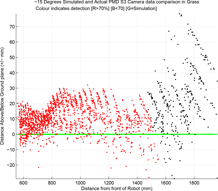
Side view comparing the simulation and actual PMD S3 data for a −15-degree mounting angle

The trend revealed by these plots is consistent throughout the angles and for the same survey that was taken of a grass surface. From close inspection of the data returned by the ToF camera, it seems that the discrepancy in performance conforms to some form of a trend. The difference in the measurements can be seen to conform to a curve down along the x and y axes. Ordinarily, this would not be significant but the data points vary from 100 mm brackets. This is significant for the AGV because it cannot traverse obstacles greater than 150 mm. If the AGV's normal conception of the ground plain consisted of consistent curves (as shown), the compilation of error would compound and lead to improper functionality. Hence, from here, an in-depth process of analysis, characterization and devising corrections was initiated.

5.2 Investigating the ToF Performance Discrepancy

The function of a ToF camera was researched in the early stages of this work; however, no risk was perceived from the point of view of the physics via which the camera functions. The error seen in the plots was attributed to a well-known phenomenon, namely ‘light scattering'.

The key difference between indoor and outdoor ToF applications was that of gaining a conception of the ground required for IR light to be incident on angles much closer to 0 degrees compared to 90 degrees. This meant the susceptibility to IR scattering needed to be considered.

Essentially, IR emitted from the ToF camera was subject to less volume-return to the receiver, thus tricking the device into thinking the distance measurements were further away. Fortunately, the difference in performance was uniform and predictable. Because of this it was possible to develop correction, thereby making the camera useful for obstacle avoidance.

5.3 Quantifying the ToF Performance Discrepancy

Several methods were used in the analysis of the camera's performance: histograms were produced for sample pixels in the HPxVP grid to ensure that normally distributed errors were present for the camera sampling. Histograms were also applied to analyse the pixel detection, which was grouped. For most angles, it could be seen that a majority of the pixels were within the >90% detection bracket and a second large group was located in the <50% bracket. Unfortunately, >70% the detected pixels (high confidence) were seen to contribute to curve up along the extremities of the detected distance in front of the camera - this consideration was important in developing the correction.

Figure 22.

Sample of the distance measurement histograms for various Ψ = −15 grass surfaces

Another method of holistic analysis was to plot the detection rate and maximum perceived distances against the camera mounting. This also enabled a direct comparison of the performance of the camera from a grass surface with a white surface. These plots are shown in Figure 23.

Figure 23.

Pixel detection simulation and actual case

In both instances, it can be seen that the detection of the pixels is considerably less in reality. The white surface can be seen to have approximately 35% less pixel detection for any given Ψ below 20 degrees; grass can be seen to have about 15% less. It is interesting to note that the grass performance is better in this measure. This is due to the intuitive fact that grass is very smooth and thus incident IR light has a much greater chance of bouncing back off an object closer to perpendicular than flat ground.

Similar to the previous plots, both drastically under perform when it comes to comparing with the simulation's expectations. In the case of the better performing grass, a maximum detected range plateau can be seen to be slightly less than 3,000 m. These two methods of analysis were useful in quantifying the difference in terms of sheer data measurements.

Figure 24.

Grass maximum detected range at angle

Following this type of quantifying analysis, the ideal camera mounting angles Ψ for the PMD S3 on P3AT and CamCube2.0 cameras on P3DX were postulated as −15 and −20 degrees respectively. Adopting this ensured that the cameras could provide an adequate conception of obstacles, maximizing the ground plane conception.

5.4 Grid-based Ground Surface Reconstruction

The ground surface from the robots’ traversed paths was devised in MATLAB and was reconstructed using captured depth frames. The Cartesian conversion of data points scattered around the area which the robot traversed is obtained by synchronizing the orientation and position of the robot platform and thus the camera, and the data captured from the PMD cameras. The grid produced for a mounting angle of −20 degrees and a grid size of 100 mm square is shown in Figure 25. The routine was coded to go for 60 seconds until the capture frames, to synchronize each to a position and orientation, and to distribute the Cartesian coordinates into squares of the grid.

Figure 25.

Surface reconstruction: grid heights perceived in the area encountered by the PMD CamCube camera at −20 degrees

6. Real-time Motion Testing

In the motion experiment, the AGV relies on the PMD camera - as a single vision sensor - to obtain information about its surroundings and to guide it to achieve its task, and it is equipped with two shaft encoders to track its position (X_rob and Y_rob) and orientation θ_veh. The experiments were performed without prior knowledge of the workspace, such as the location, velocity, orientation and number of obstacles. The range data from the PMD camera were utilised to detect and estimate the relative distances between the vehicle and the obstacles. As the camera senses the 3D coordinates of an obstacle in different frame sequences, it uses this information to detect the obstacles using a scene flow. The ego-motion of the PMD camera mounted on the AGV can be estimated by tracking features between subsequent images [49]. The ‘Good Features to Track’ feature detection algorithm [50] is used to stabilize the moving AGV by comparing two consecutive frames.

The ego-motion compensation is a transformation from the image coordinates of a previous image to that of the current image so that the effect of the ego-motion of the camera can be eliminated [257]. The feature pairs fi_t−1,fi_t, where (t_frame⁻¹) is the last image and t_frame denotes the current image, and the ego-motion of the camera can be estimated by using a transformation model. As such, we simply apply linear regression to train the constants. The next procedure is to eliminate the bad features and refine the transformation modal.

Now, the transformation model obtained is used to manipulate the whole-image pixels in order to eliminate the effect of the ego-motion of the camera. The initial minimal path is calculated by the grid-based efficient D^∗ Lite path-planning algorithm and the PMD camera provides information on the obstacles in real-time. When an obstacle is perceived via the cameras’ FoV, the AGV processes the sensor information and, if required, it can continually re-plan its path to avoid any collision until it reaches its final goal.

The goal is to plan a collision-free path for the AGV to reach its desired position by implementing the efficient D^∗ Lite algorithm on the P3DX's onboard computer. The PMD camera is used as an exteroceptive sensor with a frame rate for the scene flow of 10 fps. All the experiments were carried out without any modifications to the P3DX controller's parameter.

In this experiment, the AGV is set to travel from an initial position (X_rob, Y_rob) = (0, 0) to a goal position (9.0 m, 0), each coordinate being (X_rob, Y_rob) with X_rob and Y_rob in metres. To perceive its surroundings, it obtains information from the sensor rather than using a priori information, and it successfully avoids the three static obstacles in its path, as shown in Figures 26 and 27.

Figure 26.

Experiment (office): plot of the AGV's x-coordinates vs y-coordinates

Figure 27.

Experiment (office): indoor test with three static obstacles

7. Conclusion

The optimal deployment of a ToF-based PMD camera on an AGV is presented in this paper, the overall mission of which is to traverse the AGV from one point to another in hazardous and hostile environments without human intervention. A ToF camera is used as the key sensory device for perceiving the operating environment, the depth data of which are populated into a workspace grip map. An optimal camera mounting angle is adopted by the analysis of various cameras’ performance discrepancies. A series of still and moving tests were carried out to verify the correct sensor operation. Finally, in the real-time autonomous path-planning experiment, the AGV relied completely on its perception system to sense the operating environment and avoid static obstacles when it traversed towards its goal. In future, real-time experiments will be conducted in dynamic environments.

Footnotes

8.

The author would like to sincerely thank Mr. Daniel Salier for the MATLAB code.

1

OpenCV (Open Source Computer Vision Library) is a library of programming functions mainly aimed at real-time computer vision, developed by Intel [].

References

Patnaik

. Robot Cognition and Navigation: An Experiment with Mobile Robots. Springer Berlin Heidelberg New York, 2007.

Gomez

J. Martinez

Caballero

A. Fernandez

Varea

I. Garcia

Ruiz

L. Rodriguez

, and Gonzalez

C. Romero

. A taxonomy of vision systems for ground mobile robots. International Journal of Advanced Robotic Systems, (1729–8806), July 2014.

Everett

H. R.

. Sensors for Mobile Robots: Theory and Application. A. K. Peters, Ltd., Natick, MA, USA, 1995.

Fardi Basel Schuenert

Ullrich

, and GerdWanielik . Shape and motion-based pedestrian detection in infrared images: A multi sensor approach. In IEEE Intelligent Vehicles Symposium IV, pages 18–23, 2005.

Sgouros

Papakonstantinous , and Tsanakas

. Localized qualitative navigation for indoor environments. In IEEE International Conference on Robotics and Automation, pages 921–926, 1996.

Bertozzi Broggi Cellario Fascioli Lombardi , and Porta . Artificial vision in road vehicles. In 28th IEEE Industrial Electronics Society Annual Conf, pages 1258–1271, 2002.

Rebai

Benabderrahmane

Azouaoui

, and Ouadah

. Moving Obstacles Detection and Tracking with Laser Range Finder. In Advanced Robotics, 2009. ICAR 2009. International Conference on, pages 1–6, 2009.

Alefs

Bram

Schreiber

David

, and Clabian

Markus

. Hypothesis based vehicle detection for increased simplicity in multi sensor. In IEEE Intelligent Vehicles Symposium, pages 261–266, 2005.

Mats Ahlskog. 3d vision. Master's thesis, Department of Computer Science and Electronics, Mälardalen University, 2007.

10.

Hussmann

Ringbeck

, and Hagebeuker

. A performance review of 3d tof vision systems in comparison to stereo vision systems. In Stereo Vision (Online book publication), pages 103–120, Vienna, Austria, 2008. I-Tech Education and Publishing.

11.

May

Stefan

. 3D Time-of-Flight Ranging for Robotic Perception in Dynamic Environments. PhD thesis, Institute for Computer Science, University of Osnabrück, Germany, 2009.

12.

Ringbeck

and Hagebeuker

. A 3D Time of Flight Camera for Object Detection. PMD Technologies GmbH, Am Eichenhang 50, 57076 Siegen, Germany, 2007.

13.

Droeschel

Robust Ego-Motion Estimation with ToF Cameras. In Proceedings of the 4th European Conference on Mobile Robots, Mlini/Dubrovnik, Croatia, September 2009.

14.

Weingarten

J.W.

Gruener

, and Siegwart

. A state-of-the-art 3d sensor for robot navigation. in intelligent robots and systems. In In IEEE/RSJ Int. Conf. on Intelligent Robots and Systems, volume 3, pages 2155–2160, 2004.

15.

Yuan

Fang

Swadzba

Philippsen

Engin

Hanheide

, and Wachsmuth

. Laser-based navigation enhanced with 3d time-of-flight data. In In Robotics and Automation, ICRA'09, pages 2844–2850, 2009.

16.

Hansard

Lee

Choi

, and Horaud

R. P.

. Time of Flight Cameras: Principles, Methods, and Applications. SpringerBriefs in Computer Science. Springer, November 2012.

17.

Wiedemann

Sauer

Driewer

, and Schilling

. Analysis and characterization of the pmd camera for application in mobile robotics. In The 17thIFAC World Congress, Seoul, Korea, pages 13689–13694, 2008.

18.

Bostelman

Roger

Hong

Tsai

Madhavan

Raj

, and Weiss

Brian

. 3d range imaging for urban search and rescue robotics research. In In Safety, Security and Rescue Robotics, Workshop, 2005 IEEE International, pages 164–169, 2005.

19.

Weyrich

Klein

Laurowski

, and Wang

. Vision Based Defect Detection on 3D Objects and Path Planning for Processing. In Proceedings of the 11th WSEAS international conference on robotics, control and manufacturing technology, and 11th WSEAS international conference on Multimedia systems & signal processing, ROCOM'11/MUSP'11, pages 19–24, Stevens Point, Wisconsin, USA, 2011. World Scientific and Engineering Academy and Society (WSEAS).

20.

Huhle

Benjamin

Jenke

Philipp

, and Strasser

Wolfgang

. On-the-fly scene acquisition with a handy multi-sensor system. International Journal of Intelligent Systems Technologies and Applications, 5(3/4):255–263, 2008.

21.

Bostelman

Russo

Albus

Hong

, and Madhavan

. Applications of a 3D Range Camera Towards Healthcare Mobility Aids. In IEEE International Conference on Networking, Sensing and Control (ICNSC '06), pages 416–421, August 2006.

22.

Falie

and Buzuloiu

. Wide range time of flight camera for outdoor surveillance. In Microwaves, Radar and Remote Sensing Symposium, 2008. MRRS 2008, pages 79–82, 2008.

23.

Castaneda

Mateus

, and Navab

. Slam combining tof and high-resolution cameras. In Applications of Computer Vision (WACV), 2011 IEEE Workshop on, pages 672–678, 2011.

24.

Almansa-Valverde

Sergio

Castillo

José Carlos

, and Fernández-Caballero

Antonio

. Mobile robot map building from time-of-flight camera. Expert Syst. Appl., 39(10):8835–8843, 2012.

25.

Penne

Jochen

Schaller

Christian

Hornegger

Joachim

, and Kuwert

Torsten

. Robust real-time 3d respiratory motion detection using time-of-flight cameras. International Journal of Computer Assisted Radiology and Surgery, 3(5):427–431, 2008.

26.

May

Werner

Surmann

, and Pervolz

. 3D Time-of-Flight Cameras for Mobile Robotics. In Intelligent Robots and Systems, 2006 IEEE/RSJ International Conference on, pages 790–795, 2006.

27.

Holz

Dirk

Schnabel

Ruwen

Droeschel

David

Stückler

Jörg

, and Behnke

Sven

. Towards semantic scene analysis with time-of-flight cameras. In Solar

Javier Ruiz-del

Chown

Eric

, and Plöger

Paul G.

, editors, RoboCup 2010: Robot Soccer World Cup XIV, volume 6556, pages 121–132, Berlin, Heidelberg, 2011. Springer-Verlag.

28.

Koch

MixIn3D: 3D Mixed Reality with ToF-Camera. In Kolb

Andreas

and Koch

Reinhard

, editors, Dynamic 3D Imaging, volume 5742 of Lecture Notes in Computer Science, pages 126–141. Springer Berlin Heidelberg, 2009.

29.

Holte

M. B.

Moeslund

T. B.

, and Fihl

. View-invariant gesture recognition using 3D optical flow and harmonic motion context. Comput. Vis. Image Underst., 114(12):1353–1361, December 2010.

30.

Schwarz

L.A.

Mkhitaryan

Mateus

, and Navab

. Estimating human 3d pose from time-of-flight images based on geodesic distances and optical flow. In Automatic Face Gesture Recognition and Workshops (FG 2011), 2011 IEEE International Conference on, pages 700–706, 2011.

31.

Schwarz

Mateus

Castaneda

, and Navab

. Manifold Learning for ToF-based Human Body Tracking and Activity Recognition. In Proceedings of the British Machine Vision Conference, pages 80.1–80.11. BMVA Press, 2010. doi:10.5244/C.24.80.

32.

Henry

Krainin

Herbst

Ren

, and Fox

. RGB-D mapping Using Kinect-Style Depth Cameras for Dense 3D Modeling of Indoor Environments. 2012.

33.

Attamimi

Muhammad

Araki

Takaya

Nakamura

Tomoaki

, and Nagai

Takayuki

. Visual recognition system for cleaning tasks by humanoid robots. International Journal of Advanced Robotic Systems, 10(384), 2013.

34.

Oggier

Lustenberger

, and Charbon

. A Virtual Keyboard Based on True-3D Optical Ranging. In BMVC'05, 2005.

35.

Soutschek

Penne

Hornegger

, and Kornhuber

. 3D Gesture-based Scene Navigation in Medical Imaging Applications using Time-of-Flight Cameras. In Computer Vision and Pattern Recognition Workshops, 2008. CVPRW. IEEE Computer Society Conference on, pages 1–6, 2008.

36.

Darrell

Morency

L. P.

, and Rahimi

. Fast 3D Model Acquisition from Stereo Images. In First International Symposium on 3D Data Processing Visualization and Transmission, pages 172–176, November 2002.

37.

Cui

Schuon

Chan

Thrun

, and Theobalt

. 3D Shape Scanning with a Time-of-Flight Camera. In IEEE CVPR 10, pages 1173–1180, 2010.

38.

Distante

Diraco

, and Leone

. Active Range Imaging Dataset for Indoor Surveillance. Annals of the BMVA, London, 3:1–16, December 2010.

39.

Teizer

. 3D Range Imaging Camera Sensing for Active Safety in Construction. In Sensors in Construction and Infrastructure Management, pages 103–117. ITcon, 2008.

40.

Moeslund

T.B.

and Holte

M. B.

. Gesture Recognition using a Range Camera. Technical report, CVMT-07-01, February 2007.

41.

Conro

Shape and Deformation Measurementusing Heterodyne Range Imaging Technology. Proceedings of 12th Asia-Pacific Conference on NDT, Auckland, New Zealand, November 2006.

42.

Kahlmann

Remondino

, and Ingensand

. Calibration for Increased Accuracy of the Range Imaging Camera Swissranger. International Archives of the Photogrammetry, Remote Sensing, and Geoinformation Sciences, XXXVI(5):136–141, 2006.

43.

Möller

Kraft

Frey

Albrecht

, and Lange

. Robust 3D Measurement with PMD Sensors. PMDTechnologies GmbH, Am Eichenhang 50, D-57076, Germany., 2005.

44.

Lindner

Marvin

and Kolb

Andreas

. Lateral and Depth Calibration of PMD-Distance Sensors. In Advances in Visual Computing, volume 4292 of Lecture Notes in Computer Science, pages 524–533. Springer Berlin Heidelberg, 2006.

45.

Ramanandan

S K

. 3D ToF Camera Calibration and Image Pre-processing. Master's thesis, Deparment of Electrical Engineering and Computer Science, University of Applied Sciences Bremen, Bremen, Germany, August 2011.

46.

http://en.wikipedia.org/wiki/OpenCV. Accessed in Aug 2011.

47.

Francis

S.L.X.

Anavatti

S.G.

, and Garratt

. Reconstructing the geometry of an object using 3d tof camera. In Merging Fields Of Computational Intelligence And Sensor Technology (CompSens), 2011 IEEE Workshop On, pages 13–17, April 2011.

48.

MESA imaging. SR4000 Manual.

49.

Jung

Boyoon

and Sukhatme

Gaurav S.

. Detecting moving objects using a single camera on a mobile robot in an outdoor environment. In in International Conference on Intelligent Autonomous Systems, pages 980–987, 2004.

50.

Shi

and Tomasi

. Good features to track. In Computer Vision and Pattern Recognition, 1994. Proceedings CVPR '94., 1994 IEEE Computer Society Conference on, pages 593–600, 1994.

A ToF-Camera as a 3D Vision Sensor for Autonomous Mobile Robotics

Abstract

Keywords

1. Introduction

2. ToF-based 3D Cameras - state-of-the-art

2.1 The Basic ToF Principle

5.3 Quantifying the ToF Performance Discrepancy

Footnotes

8.

1

References