Sage Journals: Discover world-class research

Abstract

Affordances define the relationships between the robot and environment, in terms of actions that the robot is able to perform. Prior work is mainly about predicting the possibility of a reactive action, and the object's affordance is invariable. However, in the domain of dynamic programming, a robot's task could often be decomposed into several subtasks, and each subtask could limit the search space. As a result, the robot only needs to replan its sub-strategy when an unexpected situation happens, and an object's affordance might change over time depending on the robot's state and current subtask. In this paper, we propose a novel affordance model linking the subtask, object, robot state and optimal action. An affordance represents the first action of the optimal strategy under the current subtask when detecting an object, and its influence is promoted from a primitive action to the subtask strategy. Furthermore, hierarchical reinforcement learning and state abstraction mechanism are introduced to learn the task graph and reduce state space. In the navigation experiment, the robot equipped with a camera could learn the objects' crucial characteristics, and gain their affordances in different subtasks.

Keywords

cognitive robotics affordance subtask strategy hierarchical reinforcement learning state abstraction

1. Introduction

Humans can solve different tasks in a routine and very efficient way by selecting the appropriate actions or tools to obtain the desired effect. Furthermore, their skills are acquired incrementally and continuously through interactions with the world and other people. Research on human and animal behaviour has long emphasized its hierarchical structure—the divisibility of ongoing behaviour into subtask sequences, which in turn are built of simple actions. For example, a long-distance driver knows how to reach the destination following the shortest path even if some roads are unexpectedly blocked. In this paper, we discuss such cognitive skills in the context of robotics capable of acting in dynamic world and interacting with objects in a flexible way. What knowledge representations or cognitive architecture should such a biological system possess to act in such unpredictable environment? How can the system acquire task or domain-specific knowledge to be used in new situations?

To answer these questions, we resort again to the concept of affordance originated by the American psychologist J.J.Gibson [1], who defined the affordance as the potential action between the environment and organism. According to Gibson, some affordances are learned in infancy when the child experiments with external objects. Infants first notice the affordances of objects, and only later do they begin to recognize their properties, and they are active perceivers and can perceive the affordances of objects early in development.

Although Gibson does not give a specific way to learn affordances, this term has been adopted and further developed in many research fields, ranging from art design [2], human-computer interaction [3], to robot cognition [4]. Affordances play an important role in a robot's basic cognitive capabilities such as prediction and planning; however, there are two points that should be stressed now. First, the affordance is the inherent property jointly determined by the robot and environment. For instance, the climb-ability of a stair step is not only determined by the metric measure of the step height, but also the robot's leg-length. Second, the robot system must first know how to perform a number of actions and develop some perceptual capabilities before learning the affordances. Under the concept of affordance, what the robot perceives is not necessarily object names (e.g., doors, cups, desks), but the action possibilities (e.g., passable, graspable, sittable). Furthermore, the affordance of an object might change over time depending on its use, e.g., a cup might first be reachable, then graspable, and finally pourable. From the perspective of cognitive robotics, affordances are extremely powerful since they capture essential object and environment properties, in terms of the actions that the robot is able to perform, and enable the robot to be aware early of action possibilities [6].

Compared with previous research, the main contribution of this paper lies in our novel affordance model: (i) the influence of the affordance is promoted from a primitive action to the subtask strategy; (ii) an object's affordance is related with the optimal strategy of the current subtask, and it might change over time in dynamic environment; (iii) hierarchical reinforcement learning (HRL) and state abstraction mechanism could be applied to learn the subtasks simultaneously and reduce state space.

The rest of this paper is organized as follows. We start with a review of the related work in section 2. Section 3 introduces our affordance model. Section 4 describes the navigation example that is used throughout the paper. Section 5 is about the learning framework. Section 6 presents the experiment carried out in our simulation platform. Finally, we conclude this paper in section 7.

2. Related Work

In this section, we discuss affordance research in the robotics field. According to the interaction target of the robot, current research could be classified into four categories: object's manipulation affordance, object's traversability affordance, object's affordance in human-robot context, and tool's affordance. Under these affordance models, the perceptual representation is discrete or continuous, and some typical learning methods applied in the models are shown in Table 1. Affordance formalization, which could provide a unified autonomous control framework, has also gained a great deal of attention [5].

Table 1.

Typical learning method under current affordance models

Typical learning method	Affordance model	Advantages
Reinforcement learning [17, 18]	Object's manipulation affordance	Incremental learning of primitive actions, and context generalization
Bayesian network [6, 7]		Prediction and planning in bi-directional way
Statistical relational [14]		Model multi-object relationship
Ontology knowledge [15, 16]		Handle object's sudden appear or disappear
Support vector machine [9, 10, 21]	Object's manipulation and traversability affordance	Prediction and multi-step planning
Probability graphical model [19, 20]	Object's traversability affordance	Discriminative and generative model for incremental learning
Markov random field [23]	Object's affordance in human-robot context	Learn object affordances in human context from 3D data, in which the human activities span over long durations

2.1 Object's manipulation affordance

This kind of research is focused on predicting the opportunities or effects of exploratory behaviours. For instance, Montesano et al. used probabilistic network that captured the stochastic relations between objects, actions and effects. That network allowed bi-directional relation learning and prediction, but could not allow more than one step prediction [6, 7]. Hermans et al. proposed the use of physical and visual attributes as a mid-level representation for affordance prediction, and that model could result in superior generalization performance [8]. Ugur et al. encoded the effects and objects in the same feature space, their learning system shared crucial elements such as goal-free exploration and self-observation with infant development [9, 10]. Hart et al. introduced a paradigm for programming adaptive robot control strategies that could be applied in a variety of contexts, furthermore, behavioural affordances are explicitly grounded in the robot's dynamic sensorimotor interactions with its environment [11 –13]. Moldvan et al. employed recent advances in statistical relational learning to learn affordance models for multiple objects that interact with each other, and their approach could be generalized to arbitrary objects [14]. Hidayat et al. proposed affordance-based ontology for semantic robots, their model divided the robot's actions into two levels, object selection and manipulation. Based on these semantic attributes, that model could handle situations where objects appear or disappear suddenly [15,16]. Paletta et al. presented the framework of reinforcement learning for perceptual cueing to opportunities for interaction of robotic agents, and features could be successfully selected that were relevant for prediction towards affordance-like control in interaction, and they believed that affordance perception was the basis cognition of robotics [17, 18].

2.2 Object's Traversability Affordance

This kind of research is about robot traversal in large space. Sun et al. provided a probabilistic graphical model which utilized discriminative and generative training algorithms to support incremental affordance learning: their model casts visual object categorization as an intermediate inference step in affordance prediction, and could predict the traversability of terrain regions [19, 20]. Ugur et al. studied the learning and perception of traversability affordance on mobile robots and their method is useful for researchers from both ecological psychology and autonomous robotics [21].

2.3 Object's Affordance in Human-robot Context

Unlike the working environment presented above, Koppula et al. showed that human-actor based affordances were essential for robots working in human spaces in order for them to interact with objects in human desirable way [22]. They treated it as classification problem: their affordance model was based on Markov random field and could detect the human activities and object affordances from RGB-D videos. Heikkila formulated a new affordance model for astronaut-robot task communication, which could involve the robot having a human-like ability to understand the affordances in task communication [23].

2.4 Tool's Affordance

The ability to use tools is an adaptation mechanism used by many organisms to overcome the limitations imposed on them by their anatomy. For example, chimpanzees use stones to crack nuts open and sticks to reach food, dig holes, or attack predators [24]. However, studies of autonomous robotic tool use are still rare. One representative example is from Stoytchev, who formulated a behaviour-grounded computational model of tool affordances in the behavioural repertoire of the robot [25, 26].

3. Our Affordance Model

Affordance-like perception could enable the robot to react to environmental stimuli both more efficiently and autonomously. Furthermore, when planning based on an object's affordance, the robot system will be less complex and still more flexible and robust [27], and the robot could use learned affordance relations to achieve goal-directed behaviours with its simple primitive behaviours [28]. The hierarchical structure of behaviour has also been of enduring interest within neuroscience, where it has been widely considered to reflect prefrontal cortical functions. The intrinsic motivation approach to subgoal discovery in HRL dovetails with psychological theories, suggesting that human behaviour is motivated by a drive toward exploration or mastery, independent of external reward [29].

In the existing approaches, the affordance is related to only one action, and the task is finished after that action has been executed. However, sometimes the task could be divided into several subtasks, which could be described in a hierarchical graph, and the robot needs a number of actions to finish each subtask following the optimal strategy.

In this paper, we propose an affordance model as the natural mapping from the subtask, object, robot state, to the optimal action, as illustrated in Figure 1. In this model, the affordance represents the action upon the object under the optimal strategy of the current subtask. Furthermore, each subtask has its own goal, and the optimal strategy of a subtask often needs to change when an unexpected situation happens in a dynamic environment. Based on Figure 1, the formalization of our affordance model is:

Figure 1.

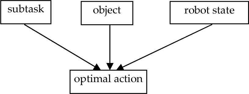
Our affordance model describes the mapping from subtask, object robot state to the optimal action that represents the first action of the optimal strategy

o p t i m a l_a c t i o n = f (s u b t a s k, ​ o b j e c t, ​ r o b o t ​ s t a t e)

(1)

Affordance prediction is a key task in autonomous robot learning, as it allows a robot to reason about the actions it can perform in order to accomplish its goals [8]. This affordance model is somewhat similar with the models proposed by Montesano and Sahin [5 –7], they all emphasize the relationship among the action, object and effect, but ours pay more attention to the goal and strategy of the subtask.

4. Navigation Example

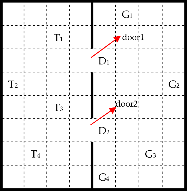
Robot navigation is a typical example where a whole task could be decomposed into several subtasks, and the robot should adjust its optimal strategy when detecting an obstacle. In this work, we use the robot navigation example to explain our affordance model. The navigation environment is shown in Figure 2: the thick black lines represent walls and they divide the eight-by-eight maze into two rooms (A, B). Each two neighbouring grids are reachable if there is no wall between them. There are four candidate trigger grids (T₁, T₂, T₃, T₄) in room A and four candidate goal grids (G₁, G₂, G₃, G₄) in room B; the start place is a random grid in room A. A trigger means that when the robot arrives at the grid, the two doors will both open immediately, as shown in Figure 3. Obstacles will appear dynamically and randomly; some could be rolled away while the others could not. The robot's task is to first navigate from the start grid to a trigger to make the doors open, then pass a door, and finally to the goal, all following the shortest routine.

Figure 2.

Initial environment

Figure 3.

The two doors are open

The robot has four primitive actions, North, South, West and East, and they are always executable. The task can be decomposed into three successive subtasks, Gototrigger, GotoDoor, and GotoGoal, which are all realized through the primitive actions. The task graph is illustrated in Figure 4, where t represents the target grid of the current subtask. Here, the goal of subtask GotoDoor is to reach grid D₁ or D₂.

Figure 4.

Task graph of the robot

The navigation process is a Markov decision process (MDP). When the robot detects an obstacle it should replan the best routine, and the affordance represents the current action, which may vary depending on the subtask and robot state. Moreover, the robot does not necessarily touch the obstacle when executing its affordance; for example, the robot may need to avoid it. As a result, the existing affordance models could not fulfill this mission; however, ours could work well.

5. The Learning Framework

HRL might be better to learn the task graph, as it is more biologically plausible. Among the existing HRL methods, MAXQ is notable because it can learn the value functions of all subtasks simultaneously—no need to wait for the value function for subtask j to converge before learning the value function for its parent task i; furthermore, a state abstraction mechanism could be applied to reduce the state space of value functions [30 –32]. As a result, we choose MAXQ as the learning method for our affordance model.

5.1 Value Function in Task Graph

Generally, the MAXQ method decomposes a MDP M into a set of subtasks {M₀, M₁, …, M_n}, M₀ is the root task, and solving it solves the entire task. The hierarchical policy π is learned for M and π = {π₀ … π_n}; each subtask M_i is a MDP and has a policy π_i.

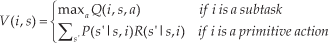
Value function Q(i, s, a) is decomposed into the sum of two components. The first is the expected total reward received while executing a, which is denoted by V (a, s). The second is completion function C(i, s, a), which describes the expected cumulative discounted reward of completing subtask M_i after invoking the subroutine for subtask M_a in state s. In MAXQ, a is a subtask or a primitive action. The optimal value function V (i, s) represents the cumulative reward of doing subtask i in state s and it can be described in (2). In this formula, P(s′ | s, i) is a probabilistic transition from state s to resulting state s′ when primitive action i is performed, R(s′ | s, i) is the reward received when primitive action i is performed and the state translates from s to s′.

V (i, ​ s) = {\begin{cases} \max_{a} Q (i, ​ s, ​ a) ​ ​ ​ ​ ​ ​ ​ ​ ​ ​ ​ ​ ​ ​ ​ i f ​ i i s a ​ s u b t a s k \\ \sum_{s'} P (s' | s, ​ i) R (s' | s, i) ​ i f i i s a ​ p r i m i t i v e ​ a c t i o n \end{cases}

(2)

The relationship between function Q, V and C is:

Q (i, ​ s, ​ a) = V (a, ​ s) + C (i, ​ s, ​ a)

(3)

The value function for the root, V(0,2), is decomposed recursively into a ser of value functions as illustrated in Equation (4):

V (0, s) = V (a_{m}, s) + C (a_{m - 1}, s, a_{m}) + \dots + C (a_{1}, s, a_{2}) + C (0, s, a_{1})

(4)

In this manner, to learn the value function of a task is substituted by a number of completion functions and primitive actions. Now, we take the first subtask GotoTrigger as an example to explain the relationship between V and C values. If the robot is in grid s and it should navigate to s₃, as shown in Figure 5, the value of this subtask is computed as follows:

Figure 5.

A sample route for subtask GotoTrigger

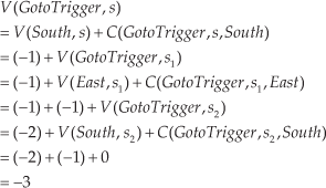
\begin{array}{l} V (G o t o T r i g g e r, ​ s) \\ = V (S o u t h, ​ s) + C (G o t o T r i g g e r, s, S o u t h) \\ = (- 1) + V (G o t o T r i g g e r, s_{1}) \\ = (- 1) + V (E a s t, s_{1}) + C (G o t o T r i g g e r, s_{1}, E a s t) \\ = (- 1) + (- 1) + V (G o t o T r i g g e r, s_{2}) \\ = (- 2) + V (S o u t h, ​ s_{2}) + C (G o t o T r i g g e r, s_{2}, S o u t h) \\ = (- 2) + (- 1) + 0 \\ = - 3 \end{array}

This process can also be represented in a tree structure as in Figure 6; the values of each C and V are shown on top of them. The reward from s to s₃ is −3, i.e., three steps are needed.

Figure 6.

Value function decomposition

5.2 Learning Algorithm

The learning algorithm is illustrated in Table 2. α_t(i) is the learning rate that could gradually be decreased, because in later stages the update speed should be increasingly slower. γ is the discount factor. 0 < α_t(i) < 1, 0 < γ ≤ 1.

Table 2.

Algorithm to learn the task graph of our affordance model

Function MAXQ (subtask i, start_state s)

{

if i is a primitive node //leaf node

execute i, receive r, and observe the result state s'

v_{t + 1} (i, ​ s) = (1 - α_{t} (i)) \cdot v_{t} (i, ​ s) + α_{t} (i) \cdot r_{t}

else

let count=0

while s is not the terminal state of subtask i, do

Choose an action a according to π(i, s)

let N=MAXQ(a, s) (recursive call)

Observe the result state s'

c_{t + 1} (i, ​ s, ​ a) = (1 - α_{t} (i)) \cdot c_{t} (i, ​ s, ​ a) + α_{t} (i) \cdot γ^{N} \cdot v_{t} (i, ​ s^{'})

count=count+N

s=s'

end // while

for all state s in subtask i

v_{t} (i, ​ s) = \max_{a} [v_{t} (a, ​ s) + c_{t} (i, ​ s, ​ a)]

End // for

End // if

}

// Main program

Initialize all v(i, s) and c(i, s, j) arbitrarily

MAXQ(subtask i, start_state s₀)

5.3 State Abstraction in Task Graph

Based on flat Q-learning, which is the standard Q-learning algorithm without subtasks, there are 64 possible states for the robot, 4 candidate trigger grids, 4 candidate goal grids and 4 executable actions; thus, we need 64×4×4×4=4096 states to represent the value functions.

GotoDoor(D₁) and GotoDoor(D₂) are different subtasks because they have different goals, then the subtask number is 4: GotoTrigger, GotoDoor(D₁), GotoDoor(D₂), GotoGoal. With subtasks but without state abstraction, a state variable contains the robot state (64), trigger position (4), target position (4), current action (4), subtask number (4), and the state number is 64×4×4×4×4=12288. Hence, we can see that without state abstraction, subtask representation requires four times the memory of a flat Q table!

In our work, two kinds of state abstractions are applied [30], one is “Subtask Irrelevance” and the other is “Leaf Irrelevance” which will be described in brief in the following section. In order to explain clearly, we draw a new task graph in Figure 7, where the state is determined by the current action, subtask number and target. The completion functions are stored in the third level. The robot's movement, with or without obstacles to avoid, is realized in terms of the four primitive actions, and the execution of the third level is ultimately transformed into the fourth level. Take N_i(t) for example (the same rule for S_i(t), W_i(t) and E_i(t)), N represents action “North”, i is the subtask number, and t is the target grid of this subtask.

Figure 7.

Task decomposition graph of our example

5.3.1 Subtask Irrelevance

Let M_i be a subtask of MDP M . A set of state variables Y is irrelevant to subtask i if the state variables of M can be partitioned into two sets X and Y such that for any stationary abstract hierarchical policy π executed by the descendants of M_i, the following two properties hold: (a) the state transition probability distribution P^π(s′, N |s, j) for each child action j of M_i can be factored into the product of two distributions :

P^{π} (x', ​ y', ​ N | x, ​ y, ​ j) = P^{π} (x', ​ N | x, ​ j) \cdot P^{π} (y' | x, ​ y, ​ j)

(5)

where x and x′ give values for the variables in X, and y and y′ give values for the variables in Y;(b) for any pair of states s₁ = (x, y₁), s₂ = (x, y₂), and any child action j, we have :

V^{π} (j, ​ s_{1}) = V^{π} (j, ​ s_{2})

(6)

In our example, the doors and final goal are irrelevant to the subtask GotoTrigger—only the current robot position and trigger point are relevant.

Take N₁(t) in subtask GotoTrigger for example; there are 32 possible positions for the robot because its working space is an eight-by-four room, and four candidate goals for the current subtask. As a result, 32×4=128 states are needed to represent N₁(t), the same result for S₁(t), W₁(t), and E₁(t), then 512 values are required for this subtask. For subtask GotoDoor, there are 32 grids and two candidate goals in room A, then 32×2=64 states are required to represent N₂(t),S₂(t), W₂(t), or E₂(t), 256 states in total. Under state abstraction, GotoDoor(D₁) and GotoDoor(D₂) have the same state space and could be included as a single subtask GotoDoor. For subtask GotoGoal, there are 32 grids and four candidate goals in room B, then 32×4=128 states are required to represent N₃(t), S₃(t), W₃(t) or E₃(t), 512 states in total. All these states are for the completion functions in the third level in Figure 5, and the total number is 512+256+512=1280.

5.3.2 Primitive Action Irrelevance

A set of state variables Y is irrelevant for a primitive action a, if for any pair of states s₁ and s₂ that differ only in their values for the variables in Y and (7) exists:

\sum_{s'_{1}} P (s'_{1} | s_{1}, ​ a) R (s'_{1} | s_{1}, ​ a) = \sum_{s'_{2}} P (s'_{2} | s_{2}, ​ a) R (s'_{2} | s_{2}, ​ a)

(7)

In our example, this condition is satisfied by the primitive actions North, South, West and East, because the reward is constant—then, only one state is required for each action. As a result, four abstract states are needed for the fourth level, and the total state space of this task graph is 1280+4=1284: far fewer than 4096, and the storage space is reduced. The essence of this abstraction is that only the related information for that state is considered. With state abstraction, the learning problem could also converge [30].

6. Experimental Validation

We test the navigation example under our own simulation environment, which is built up in C++ language, as shown in Figure 8 and Figure 9. The physical engine is Open Dynamic Engine (ODE) [33], and the render engine is Irrlicht which is an open source high performance realtime 3D engine written in C++ [34]. The floor is painted in blue or white, and any adjacent grids are in a different colour. The robot's ability includes a camera and four primitive directional actions—North, South, West, and East—and each action is deterministic. The camera could capture the front scene when the robot reaches the centre of a grid, and we can obtain the R(red), G(green), B(blue) values of each pixel in the picture.

Figure 8.

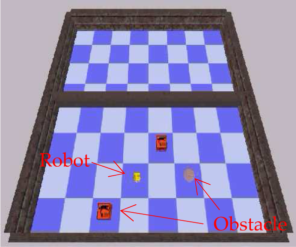
Simulation environment with robot and obstacles

Figure 9.

Simulation environment with two doors open

Because an object's affordance changes according to the current subtask it is involved in, the object's characteristics and subtask strategy should be learned first. As a result, this experiment contains three parts: (i) learn obstacles' rollable affordances in static; (ii) subtask learning without obstacles; (iii) the testing process which involves affordance calculation in a dynamic environment.

The robot and obstacles are shown in Figure 10, and the obstacles could be different in shape, colour and size. The shape includes a cube and sphere, while the size includes small, middle and large. For each state and its current subtask, there is a value(j, s) to represent the total reward of subtask j starting from state s. The policy executed during learning is a GLIE (Greedy in the Limit with Infinite Exploration) policy, which has three rules: executes each action for any state infinitely often; converges with probability 1 to a greedy policy; the recursively optimal policy is unique [32].

Figure 10.

Robot and obstacles

6.1 Affordances in Static Environment

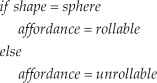
This subsection discusses the obstacles' rollable affordances in a goal-free manner in static environment, because they impact on the traversability of the preplanned routine. As this experiment is carried out in simulation environment, we restrict the size of the obstacles in a certain scope, and assume that a sphere is rollable while a cube is unrollable. As a result, the affordance in a static environment could be described in (8).

\begin{array}{l} i f ​ s h a p e = s p h e r e \\ ​ ​ ​ ​ a f f o r d a n c e = r o l l a b l e \\ e l s e ​ \\ ​ ​ ​ ​ ​ a f f o r d a n c e = u n r o l l a b l e \end{array}

(8)

The robot could detect the shape correctly with a Sobel operator and Hough transform, as illustrated in Figure 11.

Figure 11.

Obstacle detection

For (a) and (b), the left picture is what the robot captures with its own camera, and the right in blue is the detected shape. This rollable character is the basis to calculate the obstacle's affordance in a dynamic environment, and shape is the critical feature.

6.2 Subtask Learning

This subsection is to learn the optimal strategy without obstacles, and is also the basis of affordance calculations in a dynamic environment. We define the grid place as the robot's state, the execution of an action lasts from one grid's centre to the next one's centre. The reward of any primitive action is −1, but it will remain in the same place if it hits the wall or a cube. At any time, each grid could contain one obstacle at the most, and it is assumed that each obstacle will be created at the centre of a grid. The subtask graph, learning algorithm and state abstraction mechanism have been described in section 4 and 5.

In the learning process, the four triggers and goals will be chosen randomly, and the two doors could both be traversed when they are open. We have executed all the 16 pairs (Trigger_ID, Goal_ID), for simplicity we take (Trigger=T₄, Goal=G₂) as the example pair to illustrate the learning and testing result in the following part.

The learning rate α and discount factor γ are initialized as 0.9 and 1 respectively at the beginning. For every 40 episodes, the learning rate is discounted by 0.9. If γ <1, the convergence speed will be slower because the N in the learning algorithm (Table 2) is very big in the earlier training stage. The robot should finish each subtask in the shortest path, i.e., the steps from any grid to subgoal should be the smallest. In this condition, the converge of reward has the same meaning with the converge of steps. Figure 12 shows the converge result for each subtask; all the initial steps are zero. The y-axis is the step from the start grid to the current subgoal, and x-axis is the training episodes which describe the procedure that the robot finishes one subtask. The training process of (e) is based on (d) and they have intersections in learning, so (e) converges more quickly.

Figure 12.

The convergence curve diagram of steps from start to goal in each subtask

Figure 13 shows the steps from any grid to the goal in each subtask when the learning process has finished, and the number in red represents the current goal. The green numbers in (a), (b) and (c) represent the start grid in the current subtask. In (d), D₁ and D₂ could both be the start place. Take “7” in (a) for example which needs seven steps to reach the goal marked “0” in red. In (a), the four grids around the goal are all “1”, which is because each of these four grids only needs one step to reach that goal. Number “1” in (b) and (c) represents that the grids both need one step to reach goal grid D₁ or D₂. In (b) and (c), the iteration times should be large enough or the top left corner could not all be round numbers, because these grids are far to the start and goal grids and thus are visited with lower probability than the others. For D₁ and D₂, they are both inside the same subtask GotoGoal, so they can be contained in the same array as illustrated in (d).

Figure 13.

Steps from any grid to goal in each subtask

6.3 Affordances in Dynamic Environment

The testing phrase is based on the rollable characteristics and subtask strategy learned before. The affordance refers to the current action when detecting an obstacle, and their relationship is described in Table 3. For a sphere, the robot does not need to change its preplanned action even if this obstacle is on the way to the subgoal. For a cube, the robot should avoid it and choose an optimal action if this obstacle is on its way to the subgoal. If a sphere or cube is not on the robot's preplanned routine to the subgoal, the robot does not need to take care of it.

Table 3.

In this table, 1: Whether the obstacle is on the preplanned route; 2: Affordances; 3: Obstacle shape

In one example of the testing phrase, the initial places of the six obstacles created in different times are shown in Figure 14; C_i represents the ith cube and S_i represents the ith sphere. Obstacles' affordances are described in Table 4, where an obstacle's affordance changes according to the subtask it is involved in. For the robot's action selection strategy, we assume that the priority sequence of the four actions is North, South, West, East, when they have the same reward. As a result, given the start and goal, the optimal routine is sole.

Table 4.

The obstacles' affordances in different subtasks; “None” means that the obstacle could not be detected because it is not on the preplanned routine

Obstacle ID	Subtask	Action under affordance
C₁	GotoTrigger	East (unrollable)
C₂	None	No need to care
C₃	GotoGoal	East (unrollable)
S₁	GotoTrigger	South (rollable)
S₂	GotoGoal	North (rollable)
S₃	None	No need to care

Figure 14.

Obstacles' initial places

In Figure 15, (a) shows the trajectory (long grey line) without obstacle, and (b) shows the trajectory with obstacles. The grey arrow in front of the robot represents its moving direction. From the start to the trigger and then to the goal, the robot detected several obstacles and gained the correct affordances.

Figure 15.

The robot's trajectory from start to goal

Repeating the testing process many times, we can see that the robot could gain the obstacles' affordances correctly and finish the task smoothly, if the shape of the obstacle is detected exactly.

7. Conclusion

For the domain of dynamic programming, this paper presents a novel affordance model that promotes the influence of an affordance from a reactive action to the subtask strategy. An object's affordance is learned based on a subtask's optimal strategy, and the affordance might change over time. The experimental result proves that our affordance model works well in a dynamic environment.

The limitations of our model are similar with the traditional MAXQ algorithm. For example, the subtasks and their termination states should be defined by the user, and only local optimality could be learned.

In the near future, we will pay attention to three problems. The first is to introduce new algorithms that support automatic task decomposition, and gain a global optimal strategy. The second is to apply this model in a real robot and in a larger state space, but we are optimistic because the HRL and state abstraction mechanism could also be applied. The third is to generalize this affordance model to multiple robots, which should solve the problems of affordance sharing, affordance update and affordance confliction, and then the robots could be able to modify the environment and master increasingly more complex behaviours.

Footnotes

8. Acknowledgements

This work was supported by the National Natural Science Foundation of China (Grand No. 61372140)

References

Gibson

J J

(1979) The Ecological Approach to Visual Perception. Boston: Houghton Mifflin.

Hsiao

Hsu

Lee

(2012) An online affordance evaluation model for product design. Design Studies, 33(2), pp. 126–159.

Schneider

Valacich

(2011) Enhancing the motivational affordance of human-computer interfaces in a cross-cultural setting. Information Technology and Innovation Trends in Organizations, pp. 271–278.

EU Project MACS. Available at: http://www.macseu.org/. Accessed on 01 Jan 2014.

Sahin

Cakmak

Dogar

Ugur

Ucoluk

(2007) To afford or not to afford: A new formalization of affordances towards affordance-based robot control. Adaptive Behavior, 15(4), pp. 447–472.

Montesano

Lopes

Bernardino

Santos

(2008) Learning object affordances: From sensory motor coordination to imitation. IEEE Transactions on Robotics, 24(1), pp. 15–26.

Montesano

Lopes

Bernardino

Santos

(2007) Affordance, development and imitation. 2007IEEE International Conference on Development and Learning, pp. 270–275.

Hermans

Rehg

Bobick

(2011) Affordance prediction via learned object attributes. 2011 IEEE International Conference on Robotics and Automation(workshop).

Ugur

Sahin

Oztop

(2011) Unsupervised learning of object affordances for planning in a mobile manipulation platform. 2011 IEEE International Conference on Robotics and Automation, pp. 4326–4332.

10.

Ugur

Oztop

Sahin

(2011) Goal emulation and planning in perceptual space using learned affordances. Robotics and Autonomous Systems, 59(7–8), pp. 580–595.

11.

Hart

Sen

Grupen

(2008) Intrinsically motivated hierarchical manipulation, 2008 IEEE International Conference on Robotics and Automation, pp. 3814–3819.

12.

Hart

(2009) The development of hierarchical knowledge in robot systems. Ph. D. dissertation, University of Massachusetts Amherst, US.

13.

Hart

Grupen

(2011) Learning generalizable control programs. IEEE Transactions on Autonomous Mental Development, 3(3), pp. 216–231.

14.

Moldovan

Moreno

Otterlo

Santos

Raedt

(2012) Learning relational affordance models for robots in multi-object manipulation tasks. 2012 IEEE International Conference on Robotics and Automation, pp. 4373–4378.

15.

Hidayat

Kim

Ohba

(2008) Learning affordances for semantic robots using ontology. 2008 IEEE International Conference on Robotics and Automation, pp.2631–2636.

16.

Hidayat

Kim

Ohba

(2012) An approach for robots to deal with objects. International Journal of Computer Science & Information Technology, 4(1), pp. 19–32.

17.

Paletta

Fritz

(2008) Reinforcement Learning of Predictive Features in Affordance Perception. Towards Affordance-Based Robot Control. Springer- Verlag Berlin Heidelberg. pp. 77–90.

18.

Paletta

Fritz

(2007) Reinforcement learning of affordance cues. 31st workshop of the Austrian Association for Pattern Recognition. pp. 105–112.

19.

Sun

Moore

Bobick

(2010) Learning visual object categories for robot affordance prediction. The International Journal of Robotics Research, 29(2–3), pp. 174–197.

20.

Sun

(2008) Object categorization for affordance prediction. Ph. D. dissertation, Georgia Institute of Technology, US.

21.

Ugur

Sahin

(2010) Traversability: A Case study for learning and perceiving affordance in robots. Adaptive Behavior, 18(3–4), pp. 259–284.

22.

Heikkila

Halme

Schiele (2012) Affordance-based indirect task communication for astronaut-robot cooperation. Journal of Field Robotics, 29(4), pp. 576–600.

23.

Koppula

Gupta

Saxena (2013) Learning human activities and object affordances from RGBD videos. International Journal of Robotics Research. 32 (8), pp. 951–970.

24.

Beck

B B

(1980) Animal Tool Behavior: The Use and Manufacture of Tools by Animals. NY: Garland STMP Press.

25.

Stoychev

(2005) Behavior-grounded representation of tool affordances. 2005 IEEE International Conference on Robotics and Automation, pp. 3060–3065.

26.

Stoytchev

(2007) Robot Tool Behavior: A Developmental Approach to Autonomous Tool Use. Ph. D. Dissertation. Georgia Institute of Technology.

27.

Lorken

Hertzberg

(2008) Grounding planning operators by affordances. Proceeding of the 2008 International Conference on Cognitive Systems. pp. 79–84.

28.

Dogar

M R

Cakmak

Ugur

Sahin

(2007) From primitive behaviors to goal-directed behavior using affordance. IEEE/RSJ International Conference on Intelligent Robots and Systems. pp. 729–734.

29.

Botvinick

M M

Niv

Barto

A C

(2009) Hierarchically organized behavior and its neural foundations: A Reinforcement learning perspective. Cognition, 113(3), pp. 262–280.

30.

Dietterich

(2000) Hierarchical reinforcement learning with the MAXQ value function decomposition. Journal of Artificial Intelligence Research, 13(1), pp. 227–303.

31.

Dietterich

(2000) An overview of MAXQ hierarchical reinforcement learning. Proceedings of the 4th International Symposium on Abstraction, Reformulation, and Approximation, pp. 26–44.

32.

Dietterich

(2000) State abstraction in MAXQ hierarchical reinforcement learning. Advances in Neural Information Processing Systems, pp. 994–1000.

33.

http://www.ode.org/. Accessed on 01 Nov 2013.

34.

http://irrlicht.sourceforge.net/. Accessed on 01 Nov 2013.

Affordance Learning Based on Subtask's Optimal Strategy

Abstract

Keywords

1. Introduction

2. Related Work

2.1 Object's manipulation affordance

2.2 Object's Traversability Affordance

2.3 Object's Affordance in Human-robot Context

2.4 Tool's Affordance

3. Our Affordance Model

4. Navigation Example

5. The Learning Framework

5.1 Value Function in Task Graph

5.2 Learning Algorithm

5.3 State Abstraction in Task Graph

5.3.1 Subtask Irrelevance

5.3.2 Primitive Action Irrelevance

6. Experimental Validation

6.1 Affordances in Static Environment

6.2 Subtask Learning

6.3 Affordances in Dynamic Environment

7. Conclusion

Footnotes

8. Acknowledgements

References