Sage Journals: Discover world-class research

Abstract

Animals can navigate through complex environments with amazing flexibility and efficiency: they forage over large areas, quickly learning rewarding behavior and changing their plans when necessary. Some insights into the neural mechanisms supporting this ability can be found in the hippocampus (HPC)—a brain structure involved in navigation, learning, and memory. Neuronal activity in the HPC provides a hierarchical representation of space, representing an environment at multiple scales. In addition, it has been observed that when memory-consolidation processes in the HPC are inactivated, animals can still plan and navigate in a familiar environment but not in new environments. Findings like these suggest three useful principles: spatial learning is hierarchical, learning a hierarchical world-model is intrinsically valuable, and action planning occurs as a downstream process separate from learning. Here, we demonstrate computationally how an agent could learn hierarchical models of an environment using off-line replay of trajectories through that environment and show empirically that this allows computationally efficient planning to reach arbitrary goals within a reinforcement learning setting. Using the computational model to simulate hippocampal damage reproduces navigation behaviors observed in rodents with hippocampal inactivation. The approach presented here might help to clarify different interpretations of some spatial navigation studies in rodents and present some implications for future studies of both machine and biological intelligence.

Keywords

Reinforcement learning navigation hierarchical learning hippocampus cognitive map model-based learning

1. Introduction

1.1. Some features of the hippocampus’ role in navigation

The hippocampus (HPC) is a region of the brain that plays a critical role in spatial navigation and also in encoding and recalling spatial information (Burgess et al., 1998; Hartley et al., 2014). Experiments in rodents have advanced our understanding of the neural mechanisms underlying cognitive maps, spatial navigation, and their relationship to learning and memory (Chersi & Burgess, 2015). Historically, several impactful theories suggested that the HPC was crucial for acquiring and storing environmental cues into a map-like representation (Hirsh, 1974; Keefe & Nadel, 1978). Experimental evidence in support of these theories began to emerge with the adoption of the Morris water maze: a spatial navigation task in which rats or mice are trained to swim to a hidden platform in a pool using spatial cues (R. G. M. Morris, 1981). Because they cannot see the platform, animals must rely on a complex “cognitive map” of the environment to reach it. Studies that lesioned or inactivated HPC of rodents found they were impaired in the Morris water maze and showed that the HPC is necessary for the acquisition and retention of spatial information (Gidyk et al., 2021; R. G. M. Morris et al., 1982; Sutherland et al., 1982).

1.1.1. Hierarchical representation of space

Place cells are neurons that represent specific locations in an environment and become active when the animal is there. The spatial region in which a place cell fires is called its “place field.” Place fields vary in size, representing space at various scales. “Place cells” are a key feature of the hippocampus.

The spatial representation found in the HPC is hierarchical in nature, with the hierarchy organized along the dorsal/ventral hippocampal axis (Jung et al., 1994; E. I. Moser et al., 2017). At the lowest level—the dorsal end of the HPC—individual place cells can have highly specific firing patterns tuned to particular locations, providing a “high-resolution” map of the animal’s surroundings. At the ventral end of the HPC place cells operate at a larger scale, forming patterns of activity that represent larger areas and general spatial features of the environment. These multi-scale spatial representations or maps are thought to be one important input to planning and navigation processes (probably involving other brain regions) (Mehrotra & Dubé, 2023; Scleidorovich et al., 2022).

Studies that selectively lesion or inactivate dorsal or ventral HPC show that the ventral hippocampus is important for the early stages of learning in the Morris water task, essentially getting the subject into the general area where the goal can be found. Later in training, the dorsal hippocampus is critical for learning the precise location of the escape platform. This suggests that each level in the hierarchy plays a special role in spatial learning and navigation (Gruber & McDonald, 2012; McDonald et al., 2018; Ruediger et al., 2012).

1.1.2. Acquisition versus expression of navigation behaviors

Activation of the N-methyl-D-aspartate receptor (NMDAR) in the HPC has been proposed to be a key event responsible for the structural changes that occur in neurons during learning and memory formation. Chemically blocking NMDA receptors using peripheral injections of an antagonist has been shown to impair the learning of a new platform location in the Morris water maze task, but rodents were still able to recall previous locations (R. G. Morris et al., 1986). Intraventricular and intracranial injections directly into the hippocampus produce the same effect. This has led to the view that NMDAR plasticity supports the formation of spatial representations and models, that in turn support learning and execution of new behaviors (R. G. M. Morris, 2013). Importantly, it has been shown that NMDA receptor blockade does not impair learning of new behaviors in a familiar environment (though those behaviors cannot be recalled later) but does severely impair learning in a new environment (Bye & McDonald, 2019). This suggests that animals learn a model of the environment that is used in a separate planning process (possibly distributed across multiple brain regions) to learn and plan spatial behavior.

1.1.3. Limitations of lesion/inactivation studies and the opportunity for computational models

Lesion and inactivation studies have been invaluable in studying the role of the HPC in navigation, but they have limitations (Vaidya et al., 2019). Interpretation of the results is sometimes affected by the specificity in space or time of the intervention. For example, the intervention can affect nearby regions so that the results are difficult to attribute solely to the HPC. Moreover, the timing of the intervention can be important, as the HPC is thought to be involved not only in spatial information but also in encoding, consolidating, and retrieval of spatial information. Finally, there are ethical considerations of these approaches as they can be highly invasive.

These difficulties underscore the place of computational modeling in a virtuous cycle along with experimental work. Computational models can be used to test theories arising from experimental work, help interpret experimental data, and generate testable hypotheses for experimental neuroscience to investigate. This article is an example of this virtuous cycle.

1.1.4. Reinforcement learning algorithms as models of spatial learning

Reinforcement learning (RL) is a computational framework that has been extensively used to model biological learning (Botvinick et al., 2020). It models reward-driven learning, in which an agent learns to maximize its reward in an environment through trial-and-error experimentation (Sutton & Barto, 1998). Model-based RL algorithms are particularly useful for modeling spatial navigation (Bermudez-Contreras, 2021) because they learn a model or “cognitive map” of the environment, which they use to learn and execute goal-directed behavior (Botvinick & Weinstein, 2014; Daw, 2012).

1.2. Mismatches between current reinforcement learning algorithms and hippocampal observations

Reflecting on the observations from neuroscience reveals at least two areas of potential mismatch between current reinforcement learning algorithms and the brain’s approach to spatial learning. Reconciling these differences will be important as we search for a full computational account of spatial learning:

(1) Spatial learning is hierarchical in the state space. Hierarchical abstraction seems to be a key feature of encoding in the hippocampus: that is, space is seen at multiple levels of granularity (Evensmoen et al., 2015; Jung et al., 1994). This kind of abstraction can allow more computationally efficient planning. For example, walking from my current wing of the university to a neighboring wing is actually quite complex, requiring thousands of individual actions executed in the correct sequence. To compose a plan at this level would be prohibitively complex. But starting from a simplified abstract view of the problem (“I must get from this wing to the next”) guides and simplifies the composition of a plan.

A variety of types of hierarchical abstraction have been studied and modeled, including learning action hierarchies (composing sets of atomic actions into useful routines [Eysenbach et al., 2019; Solway et al., 2014; Stolle & Precup, 2002; Xia & Collins, 2021]), learning task hierarchies (composing a sequence of sub-tasks into a larger objective [Dietterich, 2000; Li et al., 2017]), and even using language as a kind of hierarchical abstraction (Frankland & Greene, 2020; Jiang et al., 2019). Some studies have considered abstraction of state or space as the hippocampus seems to do (Dayan & Hinton, 1992; Mao, 2012), but there have been fewer studies of this kind of spatial abstraction (Eppe et al., 2022; Pateria et al., 2021) and they often use manually defined state abstractions rather than considering how the abstractions could emerge in the brain (Dayan & Hinton, 1992; Eppe et al., 2019; Ma et al., 2020; Rasmussen et al., 2017). Since hierarchical abstraction of space seems to be an important feature of animal navigation (Correa et al., 2023; Evensmoen et al., 2015; Jung et al., 1994; Ruediger et al., 2012), hierarchical state abstraction may be undervalued by modern reinforcement learning algorithms. Indeed, Eppe et al. recently identified hierarchical learning as an area where current machine learning and computational models of learning still fall short of biological intelligence (Eppe et al., 2022).

(2) Model learning and action planning are separate processes. Contemporary model-based reinforcement learning algorithms learn a model of the environment or task (though usually not a hierarchical model), but the role of the model may be slightly different in these algorithms than in the brain. Popular model-based RL algorithms use a learned model of the environment to initialize a model-free policy-learning system (Nagabandi et al., 2018), help train the policy-learning system by generating simulated experiences (Chalmers et al., 2018; Feinberg et al., 2018; Ha & Schmidhuber, 2018), or simulating trajectories through the environment as part of planning and action selection (Racanière et al., 2017; Schrittwieser et al., 2020). These models capture the dynamics of how the environment behaves in terms of percepts but not the layout of the environment per se (the difference here is the difference between the questions, “if I take a step forward what will I see?” and “if I take a step forward where will I be?”). In such algorithms, the learned world model is seen as a means to a policy: the model-learning and action-planning processes are tightly coupled (which sometimes causes convergence to local optima [Ji et al., 2022]). These approaches achieve good results and undoubtedly capture some aspects of learning in the brain, but they don’t explain neuroscientific observations suggesting that animals learn a model and conduct planning as separate processes. That is, the brain assigns intrinsic value to learning a model, and the model is used for action planning downstream. Rather than contemporary RL algorithms, this reminds us of more classical, Dyna-style model-based RL algorithms (Sutton, 1991), in which model-construction and action-planning are loosely coupled.

1.3. Contributions of this article

Here, we explore the potential benefits of the principles of learning a hierarchical model of space and separately using it for planning. We propose a computational framework that embodies one possible implementation of these principles. The computational framework includes a novel and biologically plausible state-abstraction approach. We show that this prototype of animal learning produces a hierarchical abstraction of space—like that observed in the hippocampus—and allows efficient learning and planning to reach arbitrary goals. We use the framework to simulate various types of hippocampal impairment that have been studied in mice and show that the simulations reproduce behavioral deficits observed in those mice—strengthening the argument that this framework models the spatial learning and navigation process in the brain. Finally, we explore some implications and considerations for future studies of machine and biological intelligence that involve model-based learning and planning supported by the hippocampus.

2. Results

2.1. Computational setting

To focus on the fundamental concepts being explored here, our experiments use grid world problems as simple analogues of real-world navigation. A grid world consists of a grid of discrete states the agent can occupy, and the agent must learn a route through these states to reach a reward. The agent has no sensors and is only aware of its current location—thus for this study we set aside the role of vision in navigation and focus instead on the learning of a cognitive map. The grid world problem is a simple analogue of the Morris water maze task.

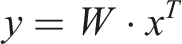
The experiments in this article cast the grid world as a Markov Decision Process and cast spatial learning and navigation as a model-based reinforcement learning problem, and we use a tabular, Dyna-like model-based learning algorithm (Poole & Mackworth, 2017) as the core learning mechanism. The algorithm maintains tables T and R that track state transitions and rewards the agent experiences, respectively. Once populated, these tables together form a model of the environment and can answer questions like “what is the probability distribution over next states after executing action a from state s.” This model can be used to calculate Q[s,a], the estimated value of executing action a from state s:

Q [s_{1}, a_{1}] = R [s_{1}, a_{1}] + γ \sum_{s_{2}} P (s_{2} | s_{1}, a_{1}) \times \underset{a_{2}}{\max Q} [s_{2}, a_{2}]

(1)

where R[s, a] (the expected reward for executing action a from state s) and P(s₂ | s, a) are estimated by the model and 𝛾 is a discount factor applied to future rewards (creating a preference for immediate rewards). This equation is applied iteratively to propagate value information throughout the states in the world (“value iteration”). To minimize computational effort, we use the prioritized sweeping algorithm (Moore & Atkeson, 1993) to apply equation (1) only to s-a pairs whose estimated value requires updating the most.

2.2. Learning a hierarchical model of the environment

Theories of how the place cell hierarchy arises in the hippocampus are varied, and the underlying mechanisms are complex (M.-B. Moser et al., 2015). Some proposals say place cells arise from the firing of grid cells (which fire in lattice patterns over an environment), but recent computational experiments have also demonstrated the reverse: that functioning place cells can give rise to grid-like cells in recurrent networks (Banino et al., 2018; Cueva & Wei, 2018; Frey et al., 2023; Sorscher et al., 2023) under some specific conditions (Schaeffer et al., 2022). Here, we take inspiration from evidence that spontaneous offline reactivation of place cells (“replay”) is an important part of spatial learning (de Lavilléon et al., 2015) and demonstrates how associations between high- and low-level place fields could arise from such reactivation.

After exploring the environment, our agent uses its learned model of the world (i.e., the state transition table T), to simulate random walks through the environment. These walks drive the aggregation of states into progressively larger macro states. The resulting hierarchical model reflects the hierarchical encoding observed in the hippocampus: with individual environment states represented at the “bottom” of the hierarchy (as in the dorsal hippocampus) and coarser regions represented at the “top” (as in the ventral hippocampus).

The aggregation process is based on a hippocampus-inspired algorithm proposed by Chalmers et al. (Chalmers et al., 2023). The architecture involves a two-layer network with the first-layer neurons representing individual places (i.e., specific or “dorsal” place cells) and the second-layer composed of winner-take-all neurons representing larger regions that aggregate multiple places. Random walks activate a particular pattern in the first-layer neurons, and the second-layer neuron that responds becomes more closely tuned to that walk’s constituent places. Since walks that occupy similar regions of space tend to overlap, and since random walks do not cross boundaries, the architecture gradually becomes tuned to clusters of places that “go together” and respect environmental structure. Thus, a meaningful abstraction emerges directly from the random walks. Here, we extend Chalmers’ original work by allowing the agent to simulate the random walks using its learned model of the environment. We further extend the two-layer architecture to multiple layers representing increasing levels of aggregation or abstraction. The result is a hierarchical abstraction of state—similar to that in the hippocampus (see Figure 1, and “Methods” section for more details).

2.3. Using the hierarchical model to plan behavior

By consulting its Q values and model, the agent can identify a previously experienced reward or goal state. At the world-level this goal may be far away, and discounting over great distance dilutes the reward signal such that the route to the goal is not clear from the current position. One solution is to increase 𝛾 and invest more energy in computation (evaluations of equation (1)) to push the reward signal back to the agent. But a hierarchical model allows a better solution: realize that at the highest level of abstraction the goal is only a few steps away (see Figure 2). Thus, information about current and goal states flows upward through the hierarchy to determine relative positioning at each level of abstraction. Plans can then be made recursively from the top down. At the highest level, a plan to reach the goal likely involves only a few transitions between macro-states. Plans to affect each of these transitions are made at the next level down, and this process repeats to the lowest (world) level. The plans are made using the same value iteration approach described above: for each planning sub-problem, an artificial reward function is created that rewards the desired transition at the given level, and prioritized sweeping is used to compute the best way to achieve the transition at that level.

Figure 1.

Learning a hierarchical model of the environment. The agent learns a low-level world model through exploration of the environment (top left). Abstract macro-states that respect environment structure emerge from simulated random walks in an unsupervised learning process (bottom row). Still higher-level abstract states emerge from the intermediate abstractions. At the highest level the abstract world model contains just four states, representing the four rooms (top right). At this level of abstraction, the goal (green dot in the original grid world) is only a few steps away from the agent (black dot), even though in the actual environment they are separated by many steps.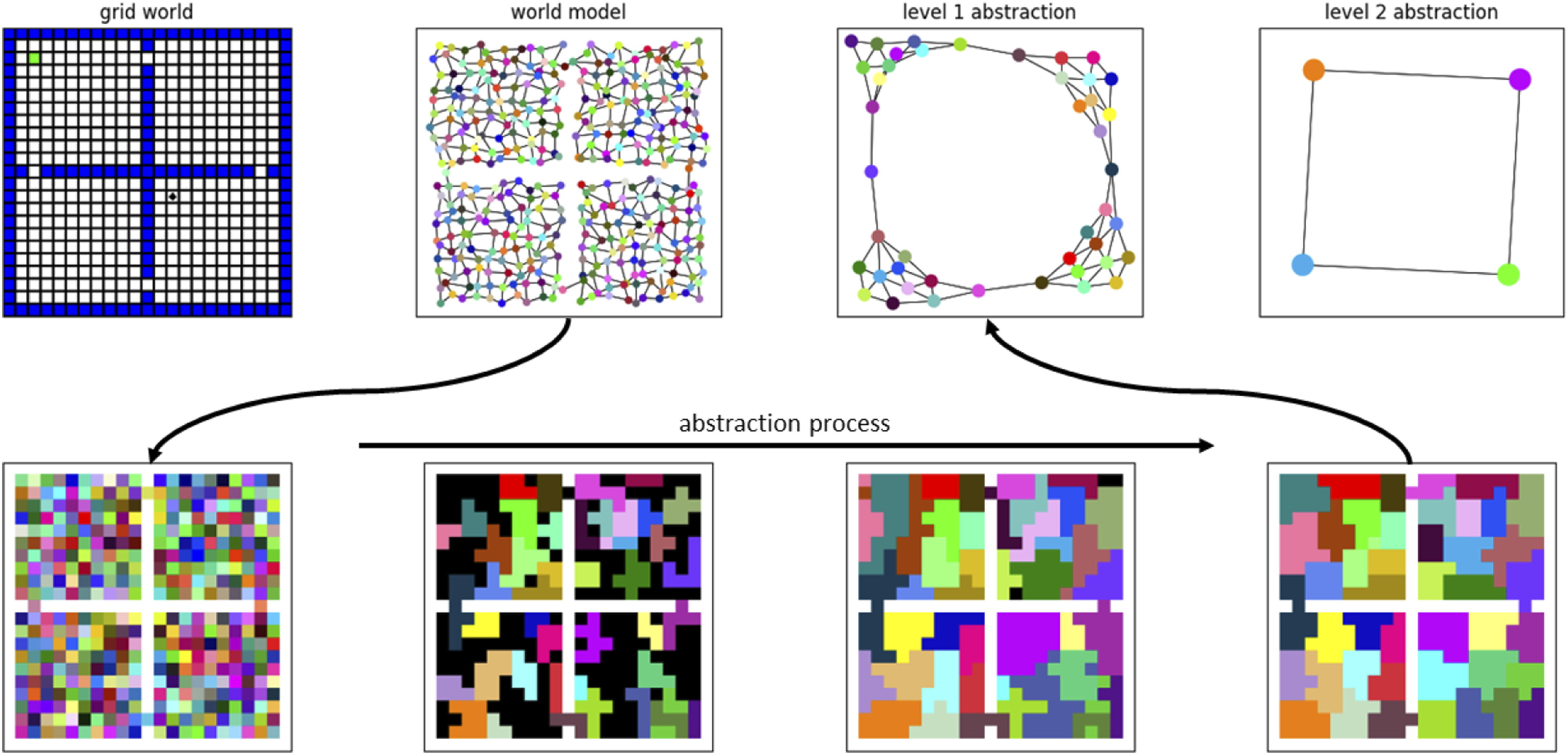

A major benefit of this hierarchical planning is that it avoids the need to propagate value information throughout a vast world model, instead focusing the calculations on a series of small sub-problems. To measure this effect, we use the hierarchical approach to solve randomly generated grid worlds and count the number of evaluations of equation (1). This count serves as a proxy for the agent’s cognitive load—the computational burden of planning rewarding actions. We compare the cognitive load of a conventional (non-hierarchical) prioritized sweeping algorithm and find that the hierarchical agent generally solves problems with less effort (Figure 2). In these experiments, all agents were allowed to self-select the 𝛾 and ϑ parameters that minimized the equation (1) calculations while still allowing them to solve the task (lower discount factor 𝛾 and higher threshold ϑ reduce the distance that value information propagates through the world model—see Methods).

Figure 2.

Hierarchical planning. At the world-level, a plan to reach the goal would involve dozens of steps. But at the highest level of abstraction—where the world consists of only four rooms—the goal is only two steps away. The first step of a plan at this level indicates an intermediate goal for the level below. The first step of a plan to reach this intermediate goal indicates an even closer intermediate goal for the level below that, and so on.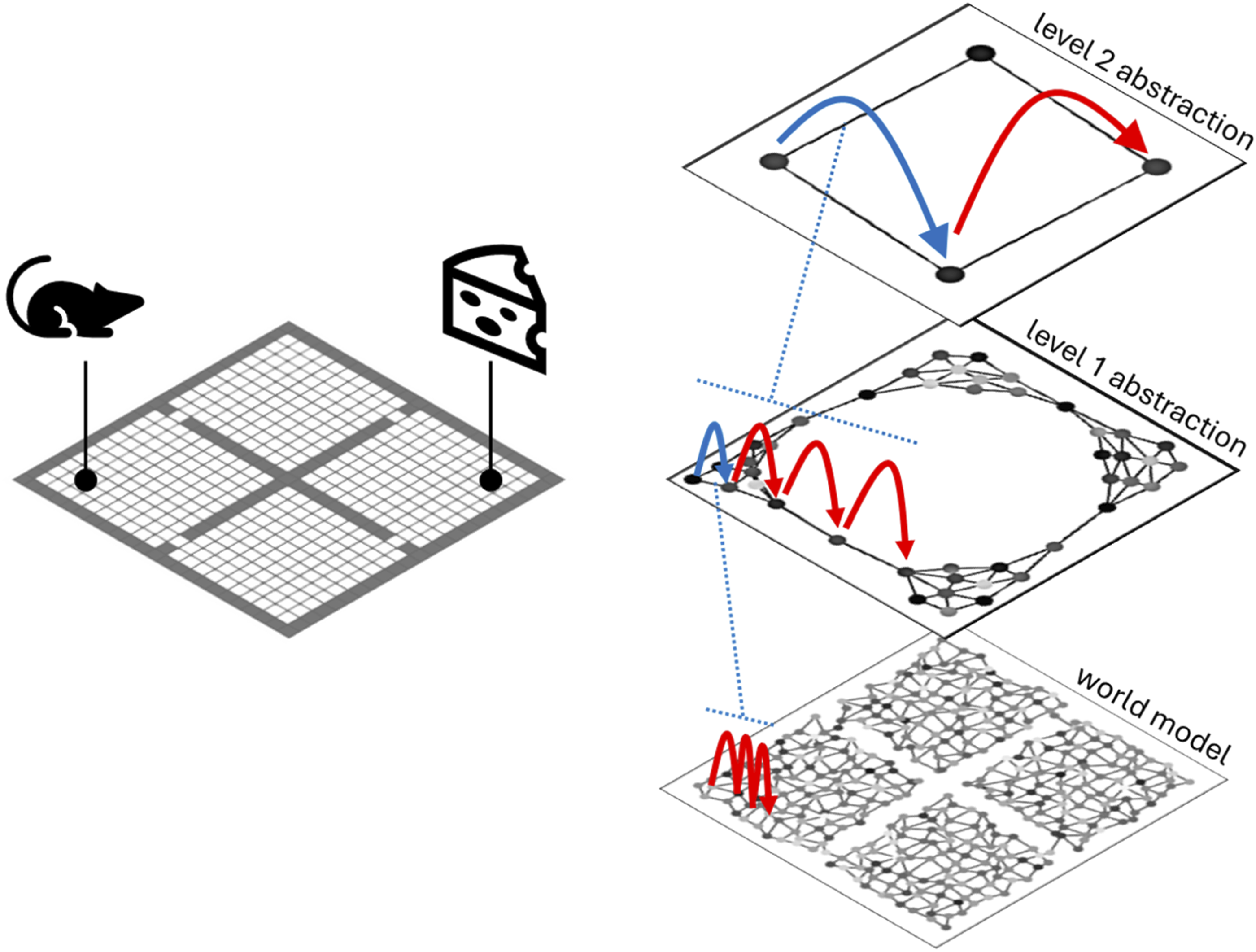

Another benefit of the hierarchical model is that it emerges from random walks in a value-agnostic way. This means that in sparse-reward, goal-seeking situations, it can be used to plan arbitrary behaviors. If the agent has been trained to perform one behavior but suddenly needs to perform a new behavior in the same environment, the new plan can be made efficiently with no additional learning. This sort of context switching would be quite difficult for a model that was tied up with value information and would be expensive without the hierarchical structure. To illustrate this, we present the conventional and hierarchical agents with a new planning problem in the environment they previously learned. The hierarchical model can create the new plan with less effort than is required by the conventional agent’s world-level value iterations. Moreover, the hierarchical plan is refined stage-by-stage, meaning the total effort is amortized over the journey, where the conventional agent must create its whole plan up-front. The trade-off is that hierarchical plans are often slightly suboptimal (Figure 3). This trade-off is probably favorable for animals who must make plans quickly and change them just as quickly when dangers arise. In this experiment, like the previous one, agents were allowed to self-select the 𝛾 and ϑ parameters that minimized the equation (1) calculations while still allowing them to solve the task.

Figure 3.

Rodents with NMDA receptors chemically blocked can plan new behaviors in familiar environments (but can’t recall them later) but cannot plan in unfamiliar environments. These observations in mice (top row, reproduced from Bye & McDonald, 2019; McDonald et al., 2005) are reproduced when NMDA blockage is simulated in our computational framework (bottom row). These effects suggest that animals learn a hierarchical model of the environment and use it (separately) for planning downstream: when a model cannot be learned, no planning is possible.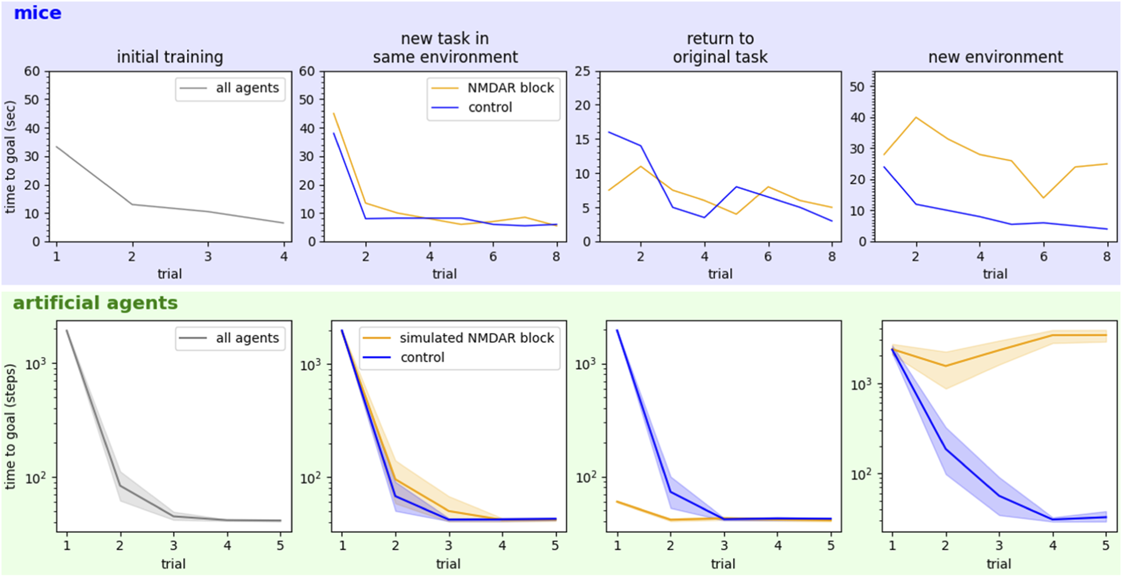

2.4. The framework reproduces observed effects of impairing hippocampus

The previous section explored the potential benefits that animals may gain by learning a hierarchical model of the world and later using it for efficient planning. This section builds credibility for the computational framework by showing that it can reproduce some important observations from neuroscience.

2.4.1. Simulating NMDAR blockage

Based on the results of blocking NMDAR in rodents, we hypothesize that NMDA is required for environment models to be learned, and also for models and planned behaviors to be stored in long-term memory. Memory consolidation in animals largely happens during rest, so we simulate periods of rest by saving our hierarchical agents’ learned models, plans, and Q values to nonvolatile memory. To simulate NMDAR block, we simply prevent both the learning of new world models and the saving of new information gained since the last simulated “rest.”

Agents with and without simulated NMDAR blockage were put through a series of four tasks similar to those used in McDonald, Bye et al. (Bye & McDonald, 2019; McDonald et al., 2005). All agents learn an original task in a novel environment. NMDAR blockage is then applied to some agents, and all learn a new task in the same environment. Agents then return to the original task—it is expected that since the blocked agents did not store the new task in long-term memory, they can resume the original task easier than agents without NMDAR blockage (controls). Finally, agents are made to learn a new task in a completely new environment. Periods of simulated rest—when the control agents save newly learned information to long-term memory—are allowed between each task.

Results are shown in Figure 3 and compared to the original observations from studies of rats with NMDAR block (Bye & McDonald, 2019; McDonald et al., 2005). Upon returning to the original task, healthy animals must relearn the rewarding behavior for that task. But the blocked animals simply resume the original behavior—they do not remember the new task that occurred in between. The blocked animals are severely impaired in the new environment because they cannot create the required world model. The computational framework reproduces both these effects.

2.4.2. Simulating partial hippocampal inactivation

Ruediger et al. studied goal-directed navigation in a water maze and found that the fine-spatial representation of the dorsal hippocampus was required for progression (over repeated trials) from random search strategies to direct swim to the goal. When the dorsal hippocampus was damaged, mice reverted to more random search strategies (Ruediger et al., 2012).

Here, we simulate damage to the dorsal hippocampus by removing a percentage of the lowest-level place fields. That is, a random subset of the lowest-level states was denied representation in the world model. The hierarchical abstractions still form from the remaining place fields, but the loss of low-level information disrupts planning. As the amount of inactivation increases, we see the same reversion to more random searching that Ruediger reported (Figure 4).

Figure 4.

Trajectories of agents with varying levels of simulated model inactivation (four sample trajectories at each of 0, 30, 50, and 80% inactivation). Agent must navigate from the black dot to the green goal. Ruediger et al. found that inactivating the dorsal hippocampus caused mice to revert to more random search strategies (Ruediger et al., 2012). Removing some states from the lowest level of the abstraction hierarchy in our framework produces a similar effect and sometimes causes navigation to fail.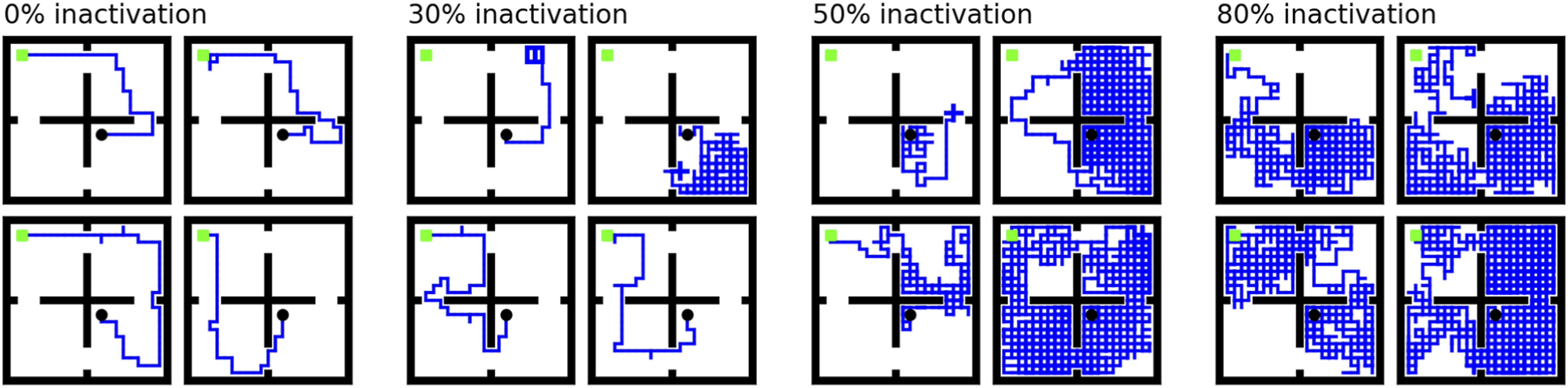

3. Discussion

In this work, we have demonstrated how an agent could learn a hierarchical representation of space as it explores its environment. This hierarchical abstraction resembles the hierarchical representation of space encoded by the hippocampus. Our experiments illustrate that a hierarchical model of an environment can be exploited for highly efficient planning and navigation. We further observe that this computational framework easily explains and reproduces key observations from hippocampal inactivation studies in rodents. Because it sees model-learning and action-planning as separate processes, the framework can explain the observation that blocking NMDAR in mice prevents them from planning in new environments, but not familiar ones: if a model of the environment cannot be learned, no planning is possible. We also reproduce a reversion to random search strategies observed by Ruediger et al. after they lesioned the dorsal hippocampus in mice: knocking out information on a subset of states in the lowest level of our abstraction framework causes a similar reversion.

3.1. Implications of our results

3.1.1. The framework captures principles of efficient, hierarchical learning and planning that the brain values

The fact that the computational framework reproduces some key results from neuroscience is evidence that this framework has captured some key aspects of how spatial learning and planning is affected in the brain. And the efficiency benefits illustrated in Figure 2 (and explored by other researchers [Correa et al., 2023; Tomov et al., 2020]) suggest why the brain works this way to begin with: If an agent can use an existing, hierarchical model for planning, it has the option to solve only the part of the environment currently of interest. In contrast, contemporary model-based algorithms that tightly couple learning and planning must often learn the world model and solve (completely) for a policy simultaneously, sometimes at great computational cost. For an animal, the ability to plan quickly is paramount. Finding food or evading a predator does not demand an optimal plan (indeed, the extra mental effort and time to arrive at a truly optimal solution may make it undesirable). Instead, the brain must find a sufficiently good solution quickly. Does achieving more human-like AI require us to trade in optimality guarantees for efficient hierarchical structures?

3.1.2. The framework makes hypotheses about place cell operation

Theories about place field formation (how place cells become associated with particular physical places) are varied, and the mechanisms are not fully understood (M.-B. Moser et al., 2015). Here, we show how offline reactivation of low-level place cells could influence the tuning of higher-level ones, giving rise to an abstraction hierarchy that respects natural divisions in the environment. But our abstraction algorithm highlights another interesting aspect of place cell learning: how relationships could form between low- and high-level place fields. That is, how a set of low-level fields representing places in a room might become associated with the high-level place field representing that room. This is an aspect of place field operation not often discussed, but these relationships are very important if the hierarchical model is indeed used for planning (to reach a particular region, one must be able to identify the individual places that would satisfy that goal). If neural recordings from rodents show this kind of association between high- and low-level place cells, that would provide further evidence that the hierarchical model supports planning processes.

3.1.3. Learning a world model is intrinsically valuable

Many contemporary model-based RL approaches learn a world model and form a policy simultaneously, and often the two processes are tightly coupled. In contrast, the brain seems to invest energy in understanding the world before it forms policies. This approach may broaden the scope of learning and support transfer between tasks. It should be a consideration in the development of new reinforcement learning algorithms.

3.1.4. Simulating hippocampal inactivation could help explain differing results among inactivation studies in rodents

Results from experimental inactivation of the hippocampus are varied. For example, some studies notice different effects when inactivating dorsal versus ventral hippocampus (Ruediger et al., 2012), while others do not (S. L. (Tommy) Lee et al., 2019). The amount of inactivation achieved affects the results (J. Q. Lee et al., 2017; Lehmann et al., 2007) and can be difficult for the experimenter to control. A computational framework like this one may help explain the varied results. By dialing up the simulated inactivation and experimenting with inactivation at different levels of the hierarchy, it may be possible to reproduce the variety of different results reported in neuroscience literature.

3.2. Limitations and open questions

While it seems this framework captures some key aspects of spatial learning and navigation in the brain, it is also clear that many other aspects remain to be integrated, or remain a mystery altogether.

3.2.1. Bottom-up, top-down, or both?

Our framework learns a model of the environment bottom-up, from world states to highest-level abstractions. In practice, it seems that ventral place fields are active quite early in learning—possibly even earlier than dorsal ones (Ruediger et al., 2012). Given only world-level information from visual and other sensors, path integration systems, and so on, how might an agent learn low-, intermediate-, and high-level abstractions all simultaneously?

3.2.2. The role of sensors in navigation and abstraction

Deep reinforcement learning algorithms have demonstrated that agents can learn complex navigation behaviors using only visual input (Mirowski et al., 2018). But Wijmans et al. demonstrated that maps emerge in the memories of agents even when they are completely blind (Wijmans et al., 2023). Here, we similarly explore behavior in agents without visual capability. In practice though, the brain makes use of both sensory input and cognitive mapping structures, and the interplay between sensation, mapping, and navigation is likely important: by moving around an animal discovers it has some control over its sensor readings, allowing their spatial meaning to be learned. Motion follows sensation and leads to learning and abstraction, which lead to efficient navigation. The older RatSLAM framework began capturing some of this complexity by integrating vision with hippocampus-like mapping (M. J. Milford et al., 2004); perhaps this type of approach should be revisited (M. Milford et al., 2016) and further integrated with modern deep reinforcement learning techniques and hierarchical planning structures.

3.2.3. What other processes does the world model support?

It seems that planning processes exist downstream from NMDA-dependent learning of a world model. That is, the model must be learned before planning can occur. If models are intrinsically valuable, they likely support other processes besides navigation planning. What might those be? Each environment model learned may somehow accelerate the learning of the next, in a meta-learning process. It is also possible that the machinery evolved in the hippocampus for solving spatial navigation problems was later reused for other kinds of perception and conceptual reasoning (Chen et al., 2022; Hawkins & Dawkins, 2021; Hawkins et al., 2018; Wu et al., 2020). If so, studying how the hippocampus learns hierarchical representations and relations of space may help us better understand (and apply, in an engineering or AI context) abstraction in other domains.

3.2.4. Tabular, Dyna-style models

Seem out of place among contemporary, deep reinforcement learning algorithms (Botvinick et al., 2020). Function approximation (e.g., through deep neural networks) is obviously necessary for scalability and generalization, and it is the almost exclusive focus of contemporary model-based RL. Yet, the hippocampus builds a cognitive map that represents discrete places explicitly—like a tabular model. How might the two approaches be combined in the brain? How should they be combined in machine learning algorithms?

3.2.5. What is the interplay between various kinds of abstraction?

Here, we focus on abstraction of space or state. As noted above, significant work has been done on other kinds of abstraction and composition of simple actions or concepts into more sophisticated ones. The brain employs many kinds of abstraction and composition at once (Eppe et al., 2022), and our framework hints at one possible avenue of cooperation between them: low-level plans made to achieve transitions between abstract states could themselves be learned as macro-actions.

3.2.6. How does the hippocampus store multiple hierarchical models?

We have shown how random walks through low-level place fields could drive a hierarchical abstraction process, tuning higher-level place fields to represent larger regions of space. The methods section below details how these associations are stored in a matrix of connection weights between low- and high-level cells. However in biology it seems that a place cell that fires in a particular location in one environment can be recruited to fire in another location in a different environment and then resume its original role when the animal returns to the original environment—a well-known “remapping” phenomenon (Colgin et al., 2008; Muller & Kubie, 1987). Our model does not currently account for this phenomenon, but we note our abstraction algorithm could be easily extended to include multiple parallel weight matrices. External context signals derived from sensory input could indicate which weight matrix is currently active—allowing multiple hierarchical models to be stored in parallel. A biological interpretation would be that multiple possible connections exist between each low- and high-level place cell, and context signals gate these connections such that different sets are enabled or suppressed in different environments, similar to Muller and Kubie’s original proposal (Muller & Kubie, 1987). Thus, the same set of place cells would learn different behaviors for different environments and switch between them appropriately. We leave exploration of this idea to future work.

3.2.7. General limitations of our abstract computational model

As scientists, we often understand complex biological systems through models (e.g., animal models, mathematical/computational models, block diagrams, and pictorial representations). Every model is a sort of metaphor: it is not the complex target system, but it has something in common with—and therefore tells us something about—that system. Like all good models, our computational model abstracts away complexity in order to highlight some general principles. In reality, navigation involves integrating information from multiple sensory processing pathways, head-direction and velocity cells, path integration, and so on. Furthermore, in reality all of this information is noisy and describes a continuous, expansive world (not a discrete grid of states as in our experiments). Our model abstracts away most of this complexity in order to highlight some fundamental principles about hierarchical model learning and planning. While it is common to use simplified reinforcement learning models this way (Bermudez-Contreras, 2021; Botvinick et al., 2020; Botvinick & Weinstein, 2014; Daw, 2012), we hope future work (our own and others’) will build more detailed models that complement (or indeed replace) this one because they include more of the complexity and can therefore say more about neurobiology.

3.3. Comparison to other abstraction-learning approaches

As mentioned in the Introduction section, we believe abstraction of space within a learning framework is somewhat understudied computationally. However, more computational accounts of the space-abstraction process itself are emerging; here, we select a few which seem particularly relevant for comparison and representative of the kinds of work being done.

Tomov et al. recently proposed an interesting Bayesian approach to state abstraction, pointing out that since the abstraction process happens offline (during rest), a more computationally intensive process is warranted. Their method of Bayesian inference over possible hierarchical abstractions produces macro-states that respect task and reward structure. Here, we follow Tomov et al. in seeing the abstraction happening offline. But we don’t suppose this means the abstraction process must be computationally demanding; here, we propose an alternative that is computationally efficient and biologically plausible.

Klukas et al. showed that an agent’s cognitive map of an environment could be partitioned into reusable abstractions based on sensory surprisal (which peaks when passing through natural environmental divisions like doorways). This provides an efficient method for online spatial abstraction. It seems likely that both online and offline abstraction mechanisms are at work in the brain, and their interplay will be an important area for future research. Here, we reproduce Klukas’ intuition that abstractions should respect environmental divisions like doorways. Klukas also illustrates the importance of re-using or sharing spatial abstractions between similar environments, which our framework would support as demonstrated previously (Chalmers et al., 2016).

Recent work by Correa et al. showed that humans create hierarchical abstractions that balance the value of a goal against the computational cost of planning. While it did not propose a specific space-abstraction method per se, Correa’s work did the important service of identifying the general principles that all hierarchical abstractions must fit within.

4. Methods

This section describes in more detail the computational methods used in our experiments. Interested readers are referred to the code repository to see more details. Of course, our implementations realize the principles discussed in this article in a computer processor: presumably the brain implements the same principles in other ways.

4.1. The model-based learning algorithm

We use a Dyna-like model-based learning algorithm (Poole & Mackworth, 2017) as the core learning mechanism in our experiments. The algorithm maintains tables T and R that track state transitions and rewards the agent experiences, respectively. Once populated, these tables together form a model of the environment and can answer questions like “what is the probability distribution over next states after executing action a from state s.” They are also used to calculate Q[s,a], the estimated value of executing action a from state s. These value calculations are applied iteratively to propagate value information throughout the states in the world (“value iteration”). To minimize computational effort, we use the prioritized sweeping algorithm (Moore & Atkeson, 1993) to prioritize calculating values that are most likely to need updating at a given time. The algorithm is described in Algorithm 1.

Algorithm 1. Pseudocode for the basic model-based learning algorithm used in our experiments.

4.2. Learning the spatial abstraction hierarchy

Our approach performs abstraction or clustering using random trajectories through the environment—inspired by the replay phenomenon in which place cell activity plays out previously experienced trajectories during rest. After the agent has explored an environment, it uses its learned model to simulate random walks through the environment. Each walk is encoded as a length-N binary vector, where N is the number of states in the environment. Each element of this vector represents a place cell assigned to a state or place in the environment, and elements representing states in the current random walk are set to one: thus, the vector can be considered a representation of low-level place cell activity for a given random walk.

These vectors create an N-dimensional space where each dimension corresponds to one state/place. Any random walk is a single point in this space, and overlapping walks will have high cosine similarity. Interestingly, all states/places are equidistant in this N-dimensional space: the vector representations for any two nodes have a cosine similarity of zero (or a Euclidean distance of 1.41) between them, regardless of how close or distant they are in the actual environment. Thus, all information about environmental structure now resides in the random walk vectors and the cosine similarities between them: walks with high cosine similarity likely come from the same region of the environment, while walks with low cosine similarly likely do not. An effective clustering can be learned on the basis of this principle.

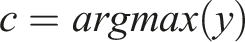
A second K-dimensional vector represents the activations of a second layer of k cells representing higher-level place fields or clusters. Connection weights between each low-level place cell and each high-level place cell are initially random. The learning process consists of identifying the “winning” high-level neuron that reacts most strongly to each random walk and incrementally strengthening its connection to the places in that walk. We model the relationship between second-layer neurons’ activity and first-layer neurons’ activity as a dot product between the input pattern and the connection weights:

y = W \cdot x^{T}

where y is the vector of second-layer neuron activations, W is a k x N sparse matrix of connection weights, with W_{i, j} being the weight of the connection between the jth first-layer neuron and ith second-layer neuron, and x is the vector of first-layer neuron activations (the input pattern).The second-layer neuron with the largest response to a given input pattern becomes more closely associated with that pattern, in winner-takes-all fashion. We model this learning process as a push of that neuron’s weights toward the input pattern. If the index of the winning neuron is denoted c:

c = argmax (y)

W_{c} + = η x

where W_c is the c^th row of W, containing the weights of connections to the winning (c^th) second-layer neuron and 𝜂 is a learning rate parameter.

So far we have been discussing a neural implementation of this abstraction or cluster-learning process. But computationally the process can be seen as an application of Online Spherical K-Means clustering (Zhong, 2005) applied in the N-dimensional random-walk space. This approach to clustering turns out to be highly data efficient and can adapt to changes in the underlying environment. For further details and experiments in a graph clustering setting, see Chalmers et al. (Chalmers et al., 2023). By repeated application of the processes (i.e., adding additional layers of cells above the second layer), we create a sequence of abstractions or clusters with increasing spatial scale, as in the hippocampus.

Each macro state created by this process has several lower-level states as constituents. To make the macro-states into a new Markov Decision Process, transitions are added to represent all possible transitions between the constituents of one macro state and the constituents of the other (per the agent’s learned model of the world). Thus each level of the hierarchy consists not only of a set of macro states or clusters but an actual MDP—an abstract version of the original MDP—in which planning can be performed.

Our computational implementation of the hierarchical abstraction process is shown in Algorithm 2.

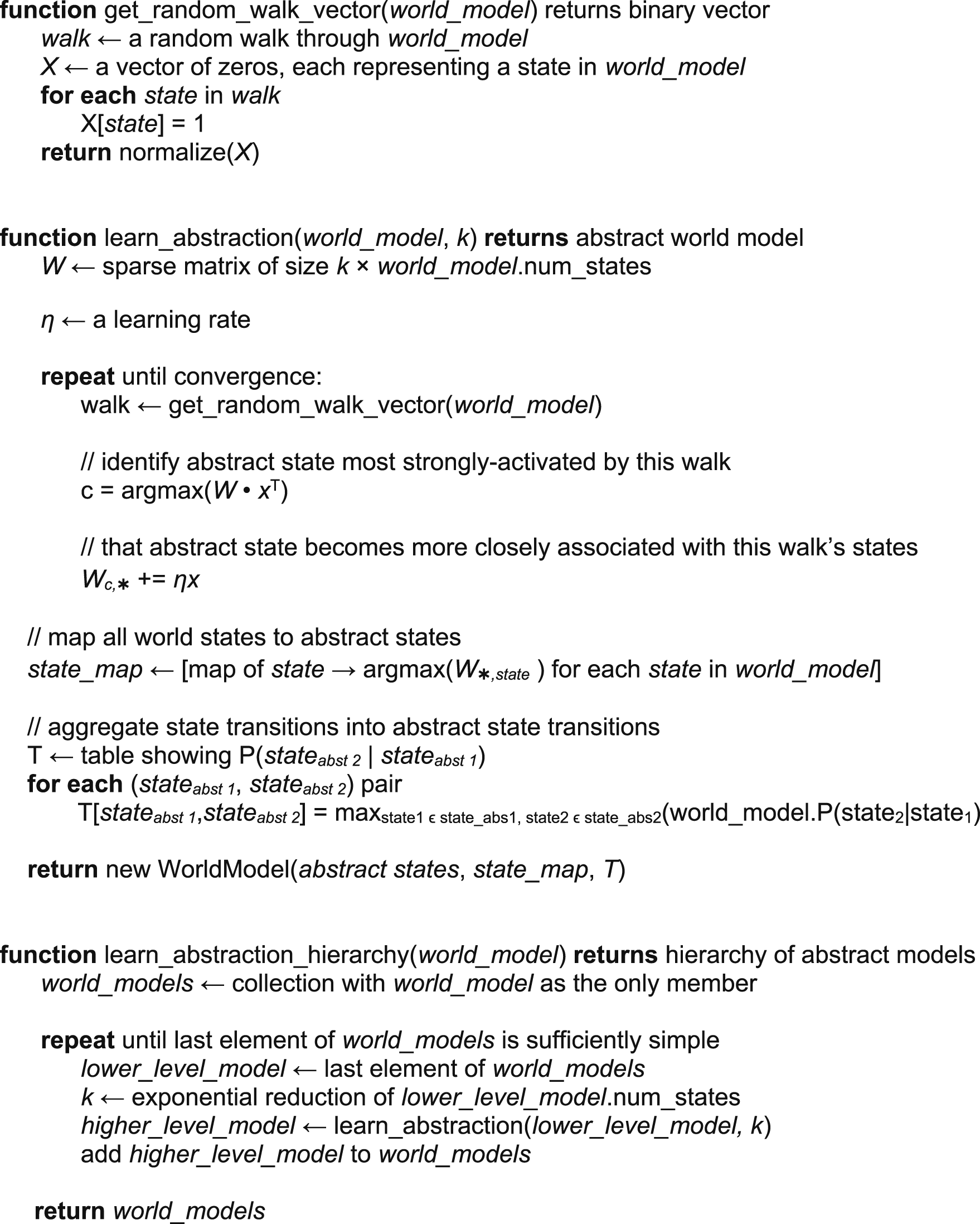
Algorithm 2. Simplified pseudo-code for the hierarchical abstraction process. For more detail, see (Chalmers et al., 2023) and the provided code repository. The world_model supplied to the learn_abstraction_hierarchy function is the model of the environment learned by the agent during its initial exploration. This algorithm creates a hierarchy of abstract models using that learned model as a base.

4.3. Hierarchical planning

If a goal in the environment (e.g., a previously experienced, high-reward state) is far away, or the environment is vast, it may be very computationally expensive to compute optimal actions using value iteration (equation (1)). Instead, the agent can resort to hierarchical abstractions learned offline to create a hierarchical plan much more efficiently, as in Tomov et al. (Tomov et al., 2020) or Chalmers et al. (Chalmers et al., 2016). While the goal may be distant at the lowest, world-level, at the highest level of abstraction it is likely only a few steps away. Value iteration can easily be applied in the high-level abstract MDP to solve the problem at that level. Then sub-problems of how to affect each high-level state transition are solved at the next level down, again using value iteration (see Algorithm 3). Since each sub-problem is significantly smaller than the full planning problem would be at that level, a hierarchical planning benefit is realized.

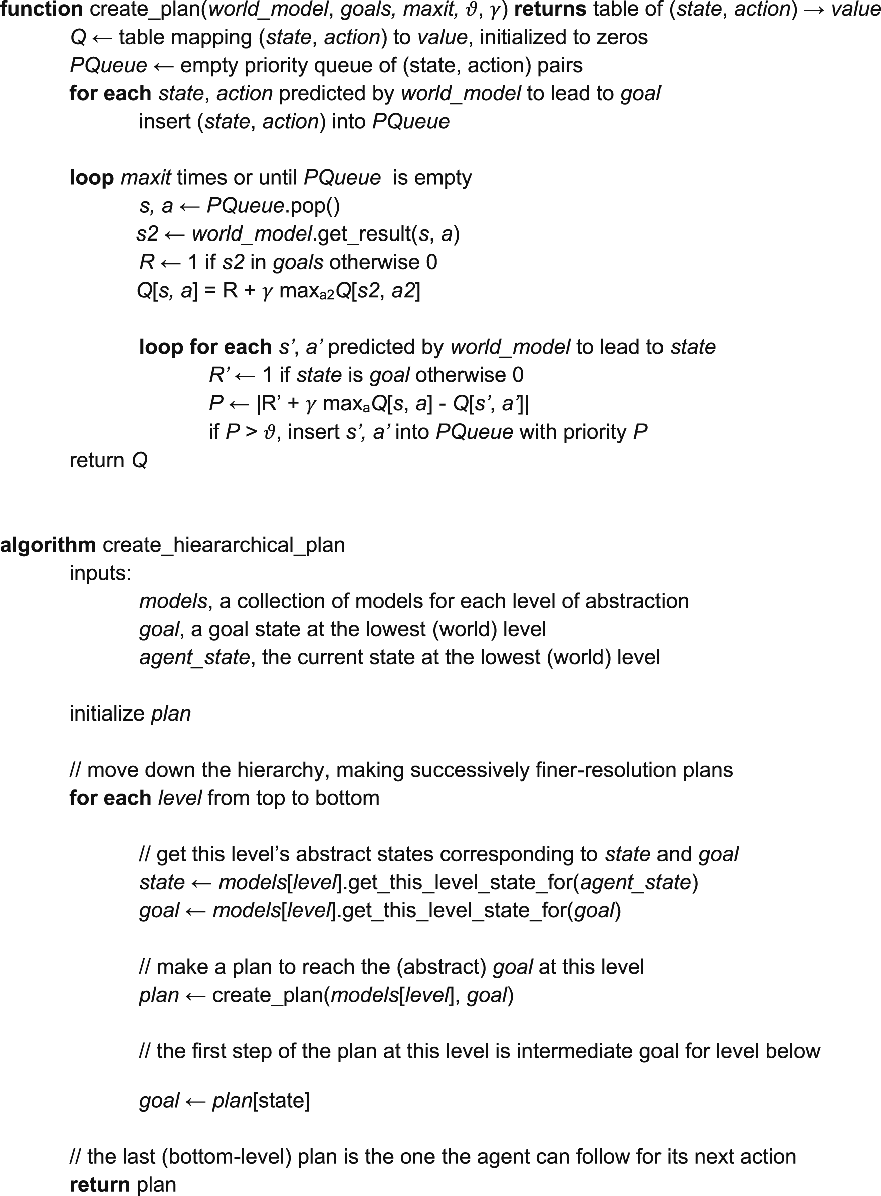
Algorithm 3: simplified pseudocode showing how the first step of a hierarchical plan can be formed. The create_plan function is essentially the prioritized sweeping algorithm (Moore & Atkeson, 1993). The create_plan step at each level of the hierarchy is planning to reach an intermediate goal determined by the cleate_plan step from the level above—since this intermediate goal is much closer than the final goal, the plans can be created with computationally conservative values for 𝜗 and 𝛾. Cross reference Figure 5.

Figure 5.

A hierarchical world model allows efficient planning. During initial learning in a randomly generated gridworld (example shown in panel b—agent must learn a route from black dot to green square), an agent with a hierarchical world model can achieve similar behavior to an agent with a flat world model but with less mental effort (panels a and d—shaded areas represent 95% confidence interval of the mean over 20 repetitions). When a new behavior is needed in a familiar environment (panel c), the hierarchical model allows efficient planning. Panel e shows the cost of planning new behavior for hierarchical-model and flat-model agents in 10 random environments: a hierarchical model allows planning with lower mental effort and amortizes that effort over the journey, whereas a flat plan must be computed up-front. The tradeoff is that hierarchical plans are sometimes suboptimal (longer).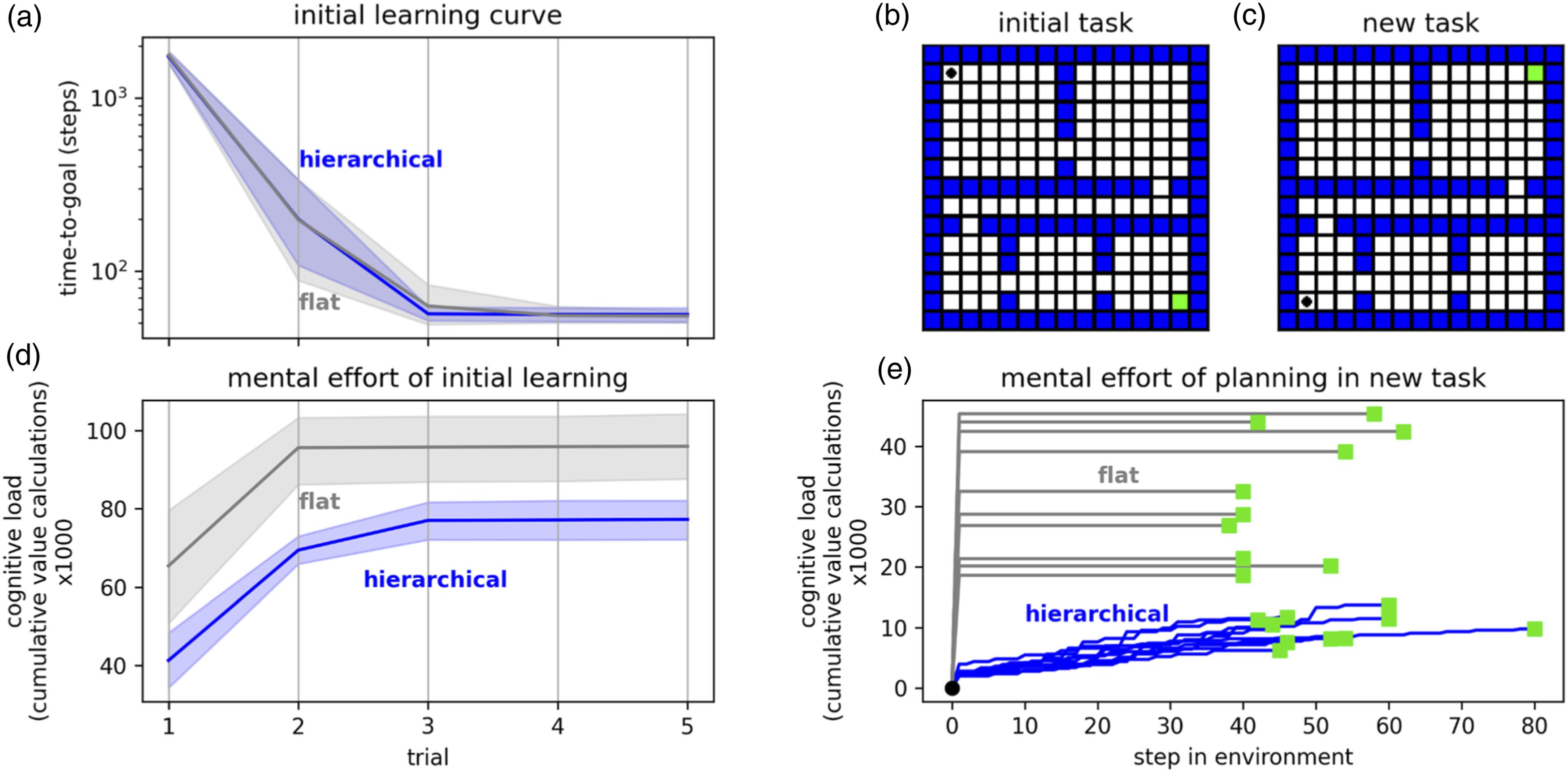

4.4. Simulating hippocampal inactivation

We simulate partial hippocampal inactivation by randomly selecting clusters of world states to deny representation in the world model, as if lesions had knocked out those particular place cells. The percentages shown in Figure 5 indicate the percentage of individual states thus affected. The table updates indicated in Algorithm 1 are skipped for these states—as a result, they cannot participate in learning or planning. Thus when the agent must venture into one of these regions it must either explore randomly or rely on sensory information about the goal, which our agent (like a mouse in a water maze) does not have.

4.5. Simulating NMDAR block and detecting changes in the environment

All of our other experiments imagine a single, standalone learning task. But for the experiments simulating NMDAR blockage, we must imagine the agent learning multiple behaviors and recalling the learned models later. In these experiments, the agents’ learned values (the Q table indicated in Algorithm 1) and world models (i.e., the T and R tables indicated in Algorithm 1), plus the hierarchical abstractions (learned per Algorithm 2), were saved (to disk) after each task and re-loaded before beginning the next task. To simulate NMDAR block, the saving-to-disk was disabled along with hierarchical model construction.

For these experiments, agents were allowed to detect changes in the task and the environment as follows: When an experienced reward did not closely match the current model’s prediction, the lowest-level model and Q values are discarded and the agent begins exploring the environment from scratch. The abstraction hierarchy is kept, however, on the assumption that this is simply a new task in the same environment. If an experienced state transition was unexpected under the current model (i.e., the probability for that transition was low), both value and dynamics information are assumed to be invalid: all models, abstractions, and Q values are discarded and the agent begins learning anew. This approach is appropriate for the sparse-reward, goal-seeking situations considered in this article and a reasonable abstraction of presumably very sophisticated change-detection mechanisms in the brain for our purposes. More sophisticated ways of comparing experience to a model may be necessary for other kinds of Markov decision processes (da Silva et al., 2006; Dick et al., 2020).

Footnotes

Declaration of conflicting interests

The author(s) declared no potential conflicts of interest with respect to the research, authorship, and/or publication of this article.

Funding

The author(s) disclosed receipt of the following financial support for the research, authorship, and/or publication of this article: The authors would like to acknowledge financial support from Mount Royal University.

Code Availability

Python code used in our experiments can be found at .

ORCID iD

Eric Chalmers

About the Authors

Eric Chalmers educated at the University of Alberta, Eric completed a BSc in Electrical Engineering and a PhD in Biomedical Engineering. Eric's current research tries to understand basic principles of intelligence and learning: understanding these principles suggests ways to better understand human intelligence (and its dysfunctions) as well as improve artificial intelligence and analytics.

Matthieu Bardal earned a BSc in Computer Science from Mount Royal University, and is now a production engineer at Shopify. In addition to AI research, Matthieu engages in all aspects of software development.

Robert McDonald received his PhD in Psychology from McGill University in Montreal, Quebec. He moved to the Department of Psychology at the University of New Mexico in 1994, completing postdoctoral training on a NSERC post-doctoral fellowship. He accepted a position at the University of Toronto in the Department of Psychology where he received tenure in 2000. He returned to the University of Lethbridge where he is currently a Full Professor. Here he has held both a Canada Research Chair and a Board of Governors Research Chair in the Department of Neuroscience. Dr. McDonald’s current research interests include: 1) developing models of the organization of learning and memory in the mammalian brain; 2) exploring plasticity mechanisms supporting hippocampal-based learning and memory functions; 3) understanding basal ganglia function and the role of specific sub- regions in goal-directed behaviour, habits, and addiction; 4) pushing boundaries of our understanding of orbitofrontal and medial prefrontal cortex function; 5) investigating the effects of pubertal drug exposure on adult cognitive function; 6) evaluating the effects of circadian dysfunction on brain and body health; 7) understanding the etiology of the sporadic form of Alzheimer’s disease; 8) developing preclinical mood disorders in rodents.

Dr. Edgar Bermudez-Contreras is the Director of AI Development at OraQ AI and an Adjunct Assistant Professor at the Neuroscience Department at the University of Lethbridge. With a PhD in Computer Science and AI from Sussex University, Dr. Bermudez has over 15 years of experience at the intersection of Computational Neuroscience and AI. His research interests range over learning, memory and spatial navigation.

References

Banino

Barry

Uria

Blundell

Lillicrap

Mirowski

Pritzel

Chadwick

M. J.

Degris

Modayil

Wayne

Soyer

Viola

Zhang

Goroshin

Rabinowitz

Pascanu

Beattie

Petersen

Kumaran

(2018). Vector-based navigation using grid-like representations in artificial agents. Nature, 557(7705), 429–433. https://doi.org/10.1038/s41586-018-0102-6

Bermudez-Contreras

(2021). Deep reinforcement learning to study spatial navigation, learning and memory in artificial and biological agents. Biological Cybernetics, 115(2), 131–134. https://doi.org/10.1007/s00422-021-00862-0

Botvinick

Wang

J. X.

Dabney

Miller

K. J.

Kurth-Nelson

(2020). Deep reinforcement learning and its neuroscientific implications. Neuron, 107(4), 603–616. https://doi.org/10.1016/j.neuron.2020.06.014

Botvinick

M.,

Weinstein

(2014). Model-based hierarchical reinforcement learning and human action control. Philosophical Transactions of the Royal Society of London. Series B, Biological Sciences, 369(1655), Article 20130480. https://doi.org/10.1098/rstb.2013.0480

Burgess

Donnett

J. G.

O’Keefe

(1998). The representation of space and the hippocampus in rats, robots and humans. Zeitschrift Fur Naturforschung. C, Journal of Biosciences, 53(7–8), 504–509. https://doi.org/10.1515/znc-1998-7-805

Bye

C. M.

McDonald

R. J.

(2019). A specific role of hippocampal NMDA receptors and arc protein in rapid encoding of novel environmental representations and a more general long-term consolidation function. Frontiers in Behavioral Neuroscience, 13, 8. https://doi.org/10.3389/fnbeh.2019.00008

Chalmers

Contreras

E. B.

Robertson

Luczak

Gruber

(2018). Learning to predict consequences as a method of knowledge transfer in reinforcement learning. IEEE Transactions on Neural Networks and Learning Systems, 29(6), 2259–2270. https://doi.org/10.1109/TNNLS.2017.2690910

Chalmers

Gruber

A. J.

Luczak

(2023). Hippocluster: An efficient, hippocampus-inspired algorithm for graph clustering. Information Sciences, 639(9), Article 118999. https://doi.org/10.1016/j.ins.2023.118999

Chalmers

Luczak

Gruber

A. J.

(2016). Computational properties of the Hippocampus increase the efficiency of goal-directed foraging through hierarchical reinforcement learning. Frontiers in Computational Neuroscience, 10, 128. https://doi.org/10.3389/fncom.2016.00128

10.

Chen

Z. S.

Zhang

Long

Zhang

S.-J.

(2022). Are grid-like representations a component of all perception and cognition? Frontiers in Neural Circuits, 16, Article 924016. https://doi.org/10.3389/fncir.2022.924016

11.

Chersi

Burgess

(2015). The cognitive architecture of spatial navigation: Hippocampal and striatal contributions. Neuron, 88(1), 64–77. https://doi.org/10.1016/j.neuron.2015.09.021

12.

Colgin

L. L.

Moser

E. I.

Moser

M.-B.

(2008). Understanding memory through hippocampal remapping. Trends in Neurosciences, 31(9), 469–477. https://doi.org/10.1016/j.tins.2008.06.008

13.

Correa

C. G.

M. K.

Callaway

Daw

N. D.

Griffiths

T. L.

(2023). Humans decompose tasks by trading off utility and computational cost. PLoS Computational Biology, 19(6), Article e1011087. https://doi.org/10.1371/journal.pcbi.1011087

14.

Cueva

C. J.

Wei

X.-X.

(2018, February 25). Emergence of grid-like representations by training recurrent neural networks to perform spatial localization. International Conference on Learning Representations. https://openreview.net/forum?id=B17JTOe0-

15.

da Silva

B. C.

Basso

E. W.

Perotto

F. S.

C Bazzan

A. L.

Engel

P. M.

(2006). Improving reinforcement learning with context detection. In 2006 Proceedings of the Fifth International Joint Conference on Autonomous Agents and Multiagent Systems, Hakodate Japan, 8–12 May, 2006, pp. 810–812. https://doi.org/10.1145/1160633.1160779

16.

Daw

(2012). Model-based reinforcement learning as cognitive search: Neurocomputational theories. https://www.semanticscholar.org/paper/Model-based-reinforcement-learning-as-cognitive-%3A-Daw/0a47d4f8d5e29a8546aba223afc692b25917efc1

17.

Dayan

P.,

Hinton

G. E.

(1992). Feudal reinforcement learning. In Advances in Neural Information Processing Systems, 5, San Francisco, CA, USA, 30 November–3 December 1992. https://papers.nips.cc/paper/1992/hash/d14220ee66aeec73c49038385428ec4c-Abstract.html

18.

de Lavilléon

Lacroix

M. M.

Rondi-Reig

Benchenane

(2015). Explicit memory creation during sleep demonstrates a causal role of place cells in navigation. Nature Neuroscience, 18(4), 493–495. https://doi.org/10.1038/nn.3970

19.

Dick

Ladosz

Ben-Iwhiwhu

Shimadzu

Kinnell

Pilly

P. K.

Kolouri

Soltoggio

(2020). Detecting changes and avoiding catastrophic forgetting in dynamic partially observable environments. Frontiers in Neurorobotics, 14, Article 578675. https://doi.org/10.3389/fnbot.2020.578675, https://www.frontiersin.org/articles/10.3389/fnbot.2020.578675

20.

Dietterich

T. G.

(2000). Hierarchical reinforcement learning with the MAXQ value function decomposition. Journal of Artificial Intelligence Research, 13, 227–303. https://doi.org/10.1613/jair.639

21.

Eppe

Gumbsch

Kerzel

Nguyen

P. D. H.

Butz

M. V.

Wermter

(2022). Intelligent problem-solving as integrated hierarchical reinforcement learning. Nature Machine Intelligence, 4(1), 11–20. https://doi.org/10.1038/s42256-021-00433-9

22.

Eppe

Nguyen

P. D. H.

Wermter

(2019). From semantics to execution: Integrating action planning with reinforcement learning for robotic causal problem-solving. Frontiers in Robotics and AI, 6, 123. https://doi.org/10.3389/frobt.2019.00123

23.

Evensmoen

H. R.

Ladstein

Hansen

T. I.

Møller

J. A.

Witter

M. P.

Nadel

Håberg

A. K.

(2015). From details to large scale: The representation of environmental positions follows a granularity gradient along the human hippocampal and entorhinal anterior-posterior axis. Hippocampus, 25(1), 119–135. https://doi.org/10.1002/hipo.22357

24.

Eysenbach

Gupta

Ibarz

Levine

(2019). Diversity is all you need: Learning skills without a reward function. International Conference on Learning Representations. https://openreview.net/forum?id=SJx63jRqFm

25.

Feinberg

Wan

Stoica

Jordan

M. I.

Gonzalez

J. E.

Levine

(2018). Model-based value estimation for efficient model-free reinforcement learning (arXiv:1803.00101). arXiv. https://doi.org/10.48550/arXiv.1803.00101

26.

Frankland

S. M.

Greene

J. D.

(2020). Concepts and compositionality: In search of the brain’s language of thought. Annual Review of Psychology, 71(1), 273–303. https://doi.org/10.1146/annurev-psych-122216-011829

27.

Frey

Mathis

M. W.

Mathis

(2023). NeuroAI: If grid cells are the answer, is path integration the question? Current Biology, 33(5), R190–R192. https://doi.org/10.1016/j.cub.2023.01.031

28.

Gidyk

D. C.

McDonald

R. J.

Sutherland

R. J.

(2021). Intact behavioral expression of contextual fear, context discrimination, and object discrimination memories acquired in the absence of the Hippocampus. Journal of Neuroscience: The Official Journal of the Society for Neuroscience, 41(11), 2437–2446. https://doi.org/10.1523/JNEUROSCI.0546-20.2020

29.

Gruber

A. J.

McDonald

R. J.

(2012). Context, emotion, and the strategic pursuit of goals: Interactions among multiple brain systems controlling motivated behavior. Frontiers in Behavioral Neuroscience, 6, 50. https://doi.org/10.3389/fnbeh.2012.00050

30.

D.,

Schmidhuber

(2018). Recurrent world models facilitate policy evolution. In Proceedings of the 32nd International Conference on Neural Information Processing Systems, 31, Montréal, Canada, 3–8 December, 2018. https://papers.nips.cc/paper_files/paper/2018/hash/2de5d16682c3c35007e4e92982f1a2ba-Abstract.html

31.

Hartley

Lever

Burgess

O’Keefe

(2014). Space in the brain: How the hippocampal formation supports spatial cognition. Philosophical Transactions of the Royal Society of London. Series B, Biological Sciences, 369(1635), Article 20120510. https://doi.org/10.1098/rstb.2012.0510

32.

Hawkins

J.,

Dawkins

(2021). A thousand brains: A new theory of intelligence. Basic Books.

33.

Hawkins

Lewis

Klukas

Purdy

Ahmad

(2018). A framework for intelligence and cortical function based on grid cells in the neocortex. Frontiers in Neural Circuits, 12, 121. https://doi.org/10.3389/fncir.2018.00121

34.

Hirsh

(1974). The hippocampus and contextual retrieval of information from memory: A theory. Behavioral Biology, 12(4), 421–444. https://doi.org/10.1016/s0091-6773(74)92231-7

35.

Luo

Sun

Jing

Huang

(2022, October 31). When to update your model: Constrained model-based reinforcement learning. Advances in Neural Information Processing Systems. https://openreview.net/forum?id=9a1oV7UunyP

36.

Jiang

(Shane) Gu

Murphy

K. P.

Finn

(2019). Language as an abstraction for hierarchical deep reinforcement learning. In Advances in Neural Information Processing Systems, 32, Vancouver, Canada, 8–14 December 2019. https://proceedings.neurips.cc/paper/2019/hash/0af787945872196b42c9f73ead2565c8-Abstract.html

37.

Jung

M. W.

Wiener

S. I.

McNaughton

B. L.

(1994). Comparison of spatial firing characteristics of units in dorsal and ventral hippocampus of the rat. Journal of Neuroscience: The Official Journal of the Society for Neuroscience, 14(12), 7347–7356. https://doi.org/10.1523/JNEUROSCI.14-12-07347.1994

38.

Keefe

J. O.,

Nadel

(1978). The hippocampus as a cognitive map. Clarendon Press.

39.

Lee

J. Q.

Sutherland

R. J.

McDonald

R. J.

(2017). Hippocampal damage causes retrograde but not anterograde memory loss for context fear discrimination in rats. Hippocampus, 27(9), 951–958. https://doi.org/10.1002/hipo.22759

40.

Lee

S. L.

(Tommy) Lew

Wickenheisser

Markus

E. J.

(2019). Interdependence between dorsal and ventral hippocampus during spatial navigation. Brain and Behavior, 9(10), Article e01410. https://doi.org/10.1002/brb3.1410

41.

Lehmann

Lacanilao

Sutherland

R. J.

(2007). Complete or partial hippocampal damage produces equivalent retrograde amnesia for remote contextual fear memories. European Journal of Neuroscience, 25(5), 1278–1286. https://doi.org/10.1111/j.1460-9568.2007.05374.x

42.

Narayan

Leong

T.-Y.

(2017). An efficient approach to model-based hierarchical reinforcement learning. Proceedings of the AAAI Conference on Artificial Intelligence, 31(1), Article 1. https://doi.org/10.1609/aaai.v31i1.11024

43.

Ouimet

Cortés

(2020). Hierarchical reinforcement learning via dynamic subspace search for multi-agent planning. Autonomous Robots, 44(3–4), 485–503. https://doi.org/10.1007/s10514-019-09871-2

44.

Mao

(2012). Hierarchical state representation and action abstractions in Q-learning for agent-based herding. International Journal of Information and Electronics Engineering. https://doi.org/10.7763/IJIEE.2012.V2.156

45.

McDonald

R. J.

Balog

R. J.

Lee

J. Q.

Stuart

E. E.

Carrels

B. B.

Hong

N. S.

(2018). Rats with ventral hippocampal damage are impaired at various forms of learning including conditioned inhibition, spatial navigation, and discriminative fear conditioning to similar contexts. Behavioural Brain Research, 351(7), 138–151. https://doi.org/10.1016/j.bbr.2018.06.003

46.

McDonald

R. J.

Hong

N. S.

Craig

L. A.

Holahan

M. R.

Louis

Muller

R. U.

(2005). NMDA-receptor blockade by CPP impairs post-training consolidation of a rapidly acquired spatial representation in rat hippocampus. European Journal of Neuroscience, 22(5), 1201–1213. https://doi.org/10.1111/j.1460-9568.2005.04272.x

47.

Mehrotra

Dubé

(2023). Accounting for multiscale processing in adaptive real-world decision-making via the hippocampus. Frontiers in Neuroscience, 17, Article 1200842. https://doi.org/10.3389/fnins.2023.1200842, https://www.frontiersin.org/articles/10.3389/fnins.2023.1200842

48.

Milford

Jacobson

Chen

Wyeth

(2016). RatSLAM: Using models of rodent Hippocampus for robot navigation and beyond. In Inaba

Corke

(Eds.), Robotics research: The 16th international symposium ISRR (pp. 467–485). Springer International Publishing. https://doi.org/10.1007/978-3-319-28872-7_27

49.

Milford

M. J.

Wyeth

G. F.

Prasser

(2004). RatSLAM: A hippocampal model for simultaneous localization and mapping. In IEEE International Conference on Robotics and Automation, 2004. Proceedings. ICRA ’04. 2004, New Orleans, LA, USA, 26 April–01 May 2004, 1, pp. 403–408. https://doi.org/10.1109/ROBOT.2004.1307183

50.

Mirowski

Grimes

Malinowski

Hermann

K. M.

Anderson

Teplyashin

Simonyan

kavukcuoglu

Zisserman

Hadsell

(2018). Learning to navigate in cities without a map. In Advances in Neural Information Processing Systems, 31, Montreal, Canada, 3–8 December 2018. https://proceedings.neurips.cc/paper_files/paper/2018/hash/e034fb6b66aacc1d48f445ddfb08da98-Abstract.html

51.

Moore

A. W.,

Atkeson

C. G.

(1993). Prioritized sweeping: Reinforcement learning with less data and less time. Machine Learning, 13(1), 103–130. https://doi.org/10.1007/BF00993104

52.

Morris

R. G.

Anderson

Lynch

G. S.

Baudry

(1986). Selective impairment of learning and blockade of long-term potentiation by an N-methyl-D-aspartate receptor antagonist, AP5. Nature, 319(6056), 774–776. https://doi.org/10.1038/319774a0

53.

Morris

R. G. M.

(1981). Spatial localization does not require the presence of local cues. Learning and Motivation, 12(2), 239–260. https://doi.org/10.1016/0023-9690(81)90020-5

54.

Morris

R. G. M.

(2013). NMDA receptors and memory encoding. Neuropharmacology, 74, 32–40. https://doi.org/10.1016/j.neuropharm.2013.04.014

55.

Morris

R. G. M.

Garrud

Rawlins

J. N. P.

O’Keefe

(1982). Place navigation impaired in rats with hippocampal lesions. Nature, 297(5868), 681–683. https://doi.org/10.1038/297681a0

56.

Moser

E. I.

Moser

M.-B.

McNaughton

B. L.

(2017). Spatial representation in the hippocampal formation: A history. Nature Neuroscience, 20(11), 1448–1464. https://doi.org/10.1038/nn.4653

57.

Moser

M.-B.

Rowland

D. C.

Moser

E. I.

(2015). Place cells, grid cells, and memory. Cold Spring Harbor Perspectives in Biology, 7(2), Article a021808. https://doi.org/10.1101/cshperspect.a021808

58.

Muller

R.,

Kubie

(1987). The effects of changes in the environment on the spatial firing of hippocampal complex-spike cells. Journal of Neuroscience: The Official Journal of the Society for Neuroscience, 7(7), 1951–1968. https://doi.org/10.1523/JNEUROSCI.07-07-01951.1987

59.

Nagabandi

Kahn

Fearing

R. S.

Levine

(2018). Neural network dynamics for model-based deep reinforcement learning with model-free fine-tuning. In 2018 IEEE International Conference on Robotics and Automation (ICRA), Brisbane, QLD, Australia, 21–25 May 2018, pp. 7559–7566. https://doi.org/10.1109/ICRA.2018.8463189

60.

Pateria

Subagdja

Tan

Quek

(2021). Hierarchical reinforcement learning: A comprehensive survey. ACM Computing Surveys, 54(5), 109.1–109.35. https://doi.org/10.1145/3453160

61.

Poole

D. L.,

Mackworth

A. K.

(2017). Artificial intelligence: Foundations of computational agents (2nd ed.). Cambridge University Press.

62.

Racanière

Weber

Reichert

Buesing

Guez

Jimenez Rezende

Puigdomènech Badia

Vinyals

Heess

Pascanu

Battaglia

Hassabis

Silver

Wierstra

(2017). Imagination-augmented agents for deep reinforcement learning. Advances in Neural Information Processing Systems, 30, Long Beach, California, US, 4–9 December 2017. https://proceedings.neurips.cc/paper/2017/hash/9e82757e9a1c12cb710ad680db11f6f1-Abstract.html

63.

Rasmussen

Voelker

Eliasmith

(2017). A neural model of hierarchical reinforcement learning. PLoS One, 12(7), Article e0180234. https://doi.org/10.1371/journal.pone.0180234

64.

Ruediger

Spirig

Donato

Caroni

(2012). Goal-oriented searching mediated by ventral hippocampus early in trial-and-error learning. Nature Neuroscience, 15(11), 1563–1571. https://doi.org/10.1038/nn.3224

65.

Schaeffer

Khona

Fiete

I. R.

(2022, May 16). No free lunch from deep learning in neuroscience: A case study through models of the entorhinal-hippocampal circuit. Advances in Neural Information Processing Systems. https://openreview.net/forum?id=syU-XvinTI1

66.

Schrittwieser

Antonoglou

Hubert

Simonyan

Sifre

Schmitt

Guez

Lockhart

Hassabis

Graepel

Lillicrap

Silver

(2020). Mastering Atari, Go, chess and shogi by planning with a learned model. Nature, 588(7839), 604–609. https://doi.org/10.1038/s41586-020-03051-4

67.

Scleidorovich

Fellous

J.-M.

Weitzenfeld

(2022). Adapting hippocampus multi-scale place field distributions in cluttered environments optimizes spatial navigation and learning. Frontiers in Computational Neuroscience, 16, Article 1039822. https://doi.org/10.3389/fncom.2022.1039822

68.

Solway

Diuk

Córdova

Yee

Barto

A. G.

Niv

Botvinick

M. M.

(2014). Optimal behavioral hierarchy. PLoS Computational Biology, 10(8), Article e1003779. https://doi.org/10.1371/journal.pcbi.1003779

69.

Sorscher

Mel

G. C.

Ocko

S. A.

Giocomo

L. M.

Ganguli

(2023). A unified theory for the computational and mechanistic origins of grid cells. Neuron, 111(1), 121–137.e13. https://doi.org/10.1016/j.neuron.2022.10.003

70.

Stolle

M.,

Precup

(2002). Learning options in reinforcement learning. In Koenig

Holte

R. C.

(Eds.), Abstraction, reformulation, and approximation (pp. 212–223). Springer. https://doi.org/10.1007/3-540-45622-8_16

71.

Sutherland

R. J.

Kolb

Whishaw

I. Q.

(1982). Spatial mapping: Definitive disruption by hippocampal or medial frontal cortical damage in the rat. Neuroscience Letters, 31(3), 271–276. https://doi.org/10.1016/0304-3940(82)90032-5

72.

Sutton

R. S.

(1991). Planning by incremental dynamic programming. In Machine learning proceedings (pp. 353–357). Elsevier.

73.

Sutton

R. S.,

Barto

A. G.

(1998). Reinforcement learning: An introduction (2nd ed.). A Bradford Book.

74.

Tomov

M. S.

Yagati

Kumar

Yang

Gershman

S. J.

(2020). Discovery of hierarchical representations for efficient planning. PLoS Computational Biology, 16(4), Article e1007594. https://doi.org/10.1371/journal.pcbi.1007594

75.

Vaidya

A. R.

Pujara

M. S.

Petrides

Murray

E. A.

Fellows

L. K.

(2019). Lesion studies in contemporary neuroscience. Trends in Cognitive Sciences, 23(8), 653–671. https://doi.org/10.1016/j.tics.2019.05.009

76.

Wijmans

Savva

Essa

Lee

Morcos

A. S.

Batra

(2023, February 1). Emergence of maps in the memories of blind navigation agents. The Eleventh International Conference on Learning Representations. https://openreview.net/forum?id=lTt4KjHSsyl

77.

C. M.

Schulz

Garvert

M. M.

Meder

Schuck

N. W.

(2020). Similarities and differences in spatial and non-spatial cognitive maps. PLoS Computational Biology, 16(9), Article e1008149. https://doi.org/10.1371/journal.pcbi.1008149

78.

Xia

L.,

Collins

A. G. E.

(2021). Temporal and state abstractions for efficient learning, transfer, and composition in humans. Psychological Review, 128(4), 643–666. https://doi.org/10.1037/rev0000295

79.

Zhong

(2005). Efficient online spherical k-means clustering. In Proceedings. 2005 IEEE International Joint Conference on Neural Networks, Montreal, QC, Canada, 31 July–04 August 2005, 5, pp. 3180–3185. https://doi.org/10.1109/IJCNN.2005.1556436

A model of how hierarchical representations constructed in the hippocampus are used to navigate through space

Abstract

Keywords

1. Introduction

1.1. Some features of the hippocampus’ role in navigation

1.1.1. Hierarchical representation of space

1.1.2. Acquisition versus expression of navigation behaviors

1.1.3. Limitations of lesion/inactivation studies and the opportunity for computational models

1.1.4. Reinforcement learning algorithms as models of spatial learning

1.2. Mismatches between current reinforcement learning algorithms and hippocampal observations

1.3. Contributions of this article

2. Results

2.1. Computational setting

2.2. Learning a hierarchical model of the environment

2.3. Using the hierarchical model to plan behavior

2.4. The framework reproduces observed effects of impairing hippocampus

2.4.1. Simulating NMDAR blockage

2.4.2. Simulating partial hippocampal inactivation

3. Discussion

3.1. Implications of our results

3.1.1. The framework captures principles of efficient, hierarchical learning and planning that the brain values

3.1.2. The framework makes hypotheses about place cell operation

3.1.3. Learning a world model is intrinsically valuable

3.1.4. Simulating hippocampal inactivation could help explain differing results among inactivation studies in rodents

3.2. Limitations and open questions

3.2.1. Bottom-up, top-down, or both?

3.2.2. The role of sensors in navigation and abstraction

3.2.3. What other processes does the world model support?

3.2.4. Tabular, Dyna-style models

3.2.5. What is the interplay between various kinds of abstraction?

3.2.6. How does the hippocampus store multiple hierarchical models?

3.2.7. General limitations of our abstract computational model

3.3. Comparison to other abstraction-learning approaches

4. Methods

4.1. The model-based learning algorithm

4.2. Learning the spatial abstraction hierarchy

4.3. Hierarchical planning

4.4. Simulating hippocampal inactivation

4.5. Simulating NMDAR block and detecting changes in the environment

Footnotes

Declaration of conflicting interests

Funding

Code Availability

ORCID iD

About the Authors

References