Formation-Based Control Scheme for Cooperative Transportation by Multiple Mobile Robots

Abstract

This paper presents a motion-planning and control scheme for a cooperative transportation system comprising a single rigid object and multiple autonomous non-holonomic mobile robots. A leader-follower formation control strategy is used for the transportation system in which the object is assumed to be the virtual leader; the robots carrying the object are considered to be followers. A smooth trajectory between the current and desired locations of the object is generated considering the constraints of the virtual leader. In the leader-follower approach, the origin of the coordinate system attached to the centre of gravity of the object, which is known as the virtual leader, moves along the generated trajectory while the real robots, which are known as followers, maintain a desired distance and orientation in relation to the leader. An asymptotically stable tracking controller is used for trajectory tracking. The proposed approach is verified by simulations and real applications using Pioneer P3-DX mobile robots.

1. Introduction

In daily life, when a person tries to carry a large and heavy object, he/she may need help from others to cooperatively transport the object. This idea may be adapted to robots for cooperative transportation tasks. Cooperative transportation has become a long-standing issue in cooperative robotics because multiple robots have potential advantages over a single robot, such as fault-tolerance, robustness and feasibility. A cooperative team of robots may perform a transportation task even if the robots experience malfunctions. They may also carry large and heavy objects in various challenging environments.

Many cooperative transportation methods for multiple robots have been introduced to evaluate cooperative transportation tasks, such as leader-follower control, the constrain-and-move strategy, the chain system, cooperative towing, and formation control. Yang et al. [1] proposed a leader-follower decentralized control system to transport a single object with non-holonomic mobile robots. A particular end-effector linked to the robot through a steering joint is used to hold and grasp the object. Zaerpoora et al. [2] introduced a decentralized method and its analysis based on a constrain-and-move strategy to transport objects. Yamaguchi and Arai [3] modelled a system including two car-like mobile robots coupled together via a carrier in two-chain and single-generator-chained form for cooperative transportation. Cheng et al. [4] presented cooperative towing of payloads by multiple mobile robots. Zhaohui et al. [5] proposed a method that allows multiple robots to work together to transport an object whose mass is not negligible, and the transportation task is viewed as a type of formation control problem.

Many cooperative transportation approaches require special equipment and mechanisms to handle an object [1, 6–10]. Moreover, the object is mostly towed or pushed cooperatively on the floor by a group of mobile robots [2], [11–14]. Robots need force distribution among them to manipulate the object during cooperative transportation [11, 15, 16]. Furthermore, some approaches in cooperative transportation utilize leader-follower-type controls [1, 6, 7, 9, 16]. Additionally, omnidirectional mobile robots or car-like mobile robots are used as carrying robots [3, 14, 16–18].

Multiple cooperating robots may be controlled by one of two approaches: centralized or decentralized. Decentralized control is more robust and scalable than centralized control [19]. Leader-follower control is applicable to decentralized control. This control approach includes one leader robot that tracks a desired trajectory, and the follower robots predict the trajectory of the leader and track it [9].

In this study, a motion-planning and control scheme for a formation-based cooperative transportation system is proposed. The system includes a single rigid object and multiple autonomous mobile robots. Each mobile robot consists of a non-holonomic mobile base with two independent driving wheels and a gripper, which is considered to be a forklift. A virtual leader-follower formation control strategy is used for the cooperative transportation system. The object to be carried is considered to be a virtual leader robot. A reference coordinate system of the virtual robot is attached to the centre of gravity of the object. A path is generated for the virtual robot. The follower robots track their paths, which are generated to maintain the formation. The shape of the formation depends on the shape of the object and grasping points of the object by the robots. Additionally, a forklift-type constraint is used to restrict the relative orientation between the virtual leader and each follower robot. This constraint is used to generate the trajectory. For the trajectory tracking, an asymptotically stable tracking control proposed by Kanayama et al. [20] and a sliding-mode tracking controller proposed by Jun et al. [21] are used comparatively. If the robots are able to track the trajectories with small tracking errors, the proposed method will not require a dynamic model of the multi-body system, and there is no need to determine the force distribution that should be applied by each follower. Simulations and real-world applications are implemented to verify the effectiveness of the proposed system. Additionally, a performance comparison of two types of tracking controller is performed for various formation types and different translational velocities of the virtual leader. Real-world applications are examined to show that the proposed formation-based cooperative transportation system makes it possible to transport an object with multiple robots. As regards the motivation of this study, we believed that the idea of applying the formation-based control scheme to the cooperative transportation problem was an original one, and that if we could show the methodology and applicability of this scheme it would represent an important contribution to the literature.

Figure 1.

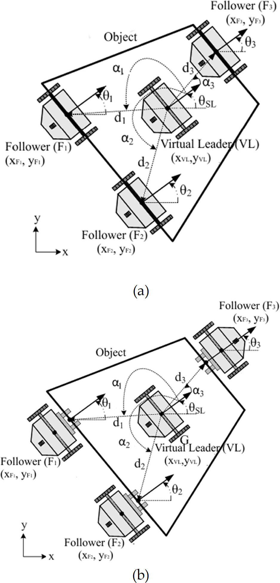
Cooperative Transportation System: (a) object over the heads, (b) object on forks

The paper is organized as follows: Section 2 introduces the proposed cooperative transportation system. In Section 3, the motion-planning scheme for the cooperative transportation system is addressed, and Section 4 presents the asymptotically stable tracking control and sliding-mode control approaches for formation control of followers. In Section 5, transportation experiments in both real and simulation environments are given. The conclusion is given in Section 6.

2. Cooperative Transportation System

The cooperative transportation system organizes the mobile robots to transfer the object from an initial location to a desired one based on the virtual leader-follower formation control strategy. The object is considered to be the virtual leader (VL), and the robots carrying the object are considered to be the followers (Fi, i=1,2,…,n), as illustrated in Figure 1. The centre of gravity of the object follows the path generated by considering the constraints of the robots.

The centre of gravity of the object, G, is located at the midpoint (x_VL, y_VL) of the VL's differential wheels. The VL has the same orientation, θ_VL, as the object. A motion plan is generated for the VL by each follower. Then, each follower determines its own trajectory according to the VL's motion plan. The followers use an inter-robot communication framework, the Open Agent Architecture (OAA) [22], to identify the nodes and the initial and final posture of the VL, and to synchronize their motions. Once the robots are synchronized, they behave in a distributed manner and maintain a formation with respect to the VL with a distance of d_i and an angle of α_i (i=1,2,…) for the i^th follower. If the followers carry the object over their heads, as observed in Figure 1a, the centre of gravity of each follower is considered to be (x_Fi, y_Fi) and to have an orientation θ_i with respect to the global coordinates. Otherwise, if the followers carry the object on their forks, as observed in Figure 1b, the centre of each follower's forks is considered to be (x_Fi, y_Fi) and to have an orientation θ_i with respect to the global coordinates. Note that one of the followers moves backward while carrying the object for the configuration observed in the figures. Furthermore, the number of followers needed to transport a rigid object may be determined based on the weight, shape, and dimension of the object. The contact points between the followers and the object may be identified by providing the equilibrium of the object. These are topics for further research.

The proposed approach can be applied to a transportation system if the following assumptions are met:

• Multiple differential non-holonomic mobile robots transport a rigid object.

• The object is transported in a two-dimensional plane over approximately smooth ground.

• During the transportation, each mobile robot knows its position and orientation, which is determined internally or externally.

• An inter-robot communication framework exists.

• The coordinate axes towards the translational motion of each follower are initially parallel because the followers are non-holonomic; however, a small deflection may be tolerated while transporting.

3. Motion Planning Scheme

For a transportation task, there is a need to generate a continuous trajectory from the current position and orientation to desired position and orientation of the object by avoiding contact with the obstacles and considering dynamic constraints of the system. It is well known that the differential-drive mobile robot is a non-holonomic system because there are differential constraints that cannot be completely integrated [23]. To generate a smooth path, first of all the kinematic model of the differential-drive mobile robot needs to be obtained.

3.1 Kinematic Model

In this study, Pioneer P3-DX mobile robot platforms with differential-drives are used. A picture of the platforms and their parameters are shown in Figure 2, respectively. They have two standard wheels and a caster wheel placed in the rear to balance the platform.

The kinematic equations of WMR are

$$\begin{array}{l}{\upsilon }_x=r\frac{\left({\upsilon }_R+{\upsilon }_L\right)}{2}\cos {\theta }_R\\ {\upsilon }_y=r\frac{\left({\upsilon }_R+{\upsilon }_L\right)}{2}\sin {\theta }_R\\ \omega =\frac{r}{D}\left({\upsilon }_R-{\upsilon }_L\right)\\ {\upsilon }_T=\frac{\left({\upsilon }_R+{\upsilon }_L\right)}{2}\end{array}$$

(1)

where D is the distance between the left and right wheels, r is the radius of the wheel, v _x and v _y are the projection of the translational velocity v _T , v _R and v _L are the velocities of right and left wheels, v _T and ω are the translational and angular velocities of the robot.

Using Equation (1), the kinematic model of the WMR can be expressed as follows:

$$\left[\begin{array}{c}{\upsilon }_x\\ {\upsilon }_y\\ \omega \end{array}\right]=\left[\begin{array}{cc}\cos {\theta }_R& 0\\ \sin {\theta }_R& 0\\ 0& 1\end{array}\right]\left[\begin{array}{c}{\upsilon }_T\\ \omega \end{array}\right]$$

(2)

If v_R is different from u_L, the robot turns in either the clockwise or anti-clockwise direction depending on the relative velocities of the two wheels. Thus, an ICC (Instantaneous Centre for Curvature) is generated, as shown in Figure 3. R is the radius of the curved path tracked by the mobile robot. The relationship between the radius of the curvature and two-wheel velocities is expressed as follows:

$$\begin{array}{l}R=r\frac{{\upsilon }_T}{\omega }\\ R=r\frac{D}{2}\left(\frac{{\upsilon }_R+{\upsilon }_L}{{\upsilon }_R-{\upsilon }_L}\right)\end{array}$$

(3)

Figure 2.

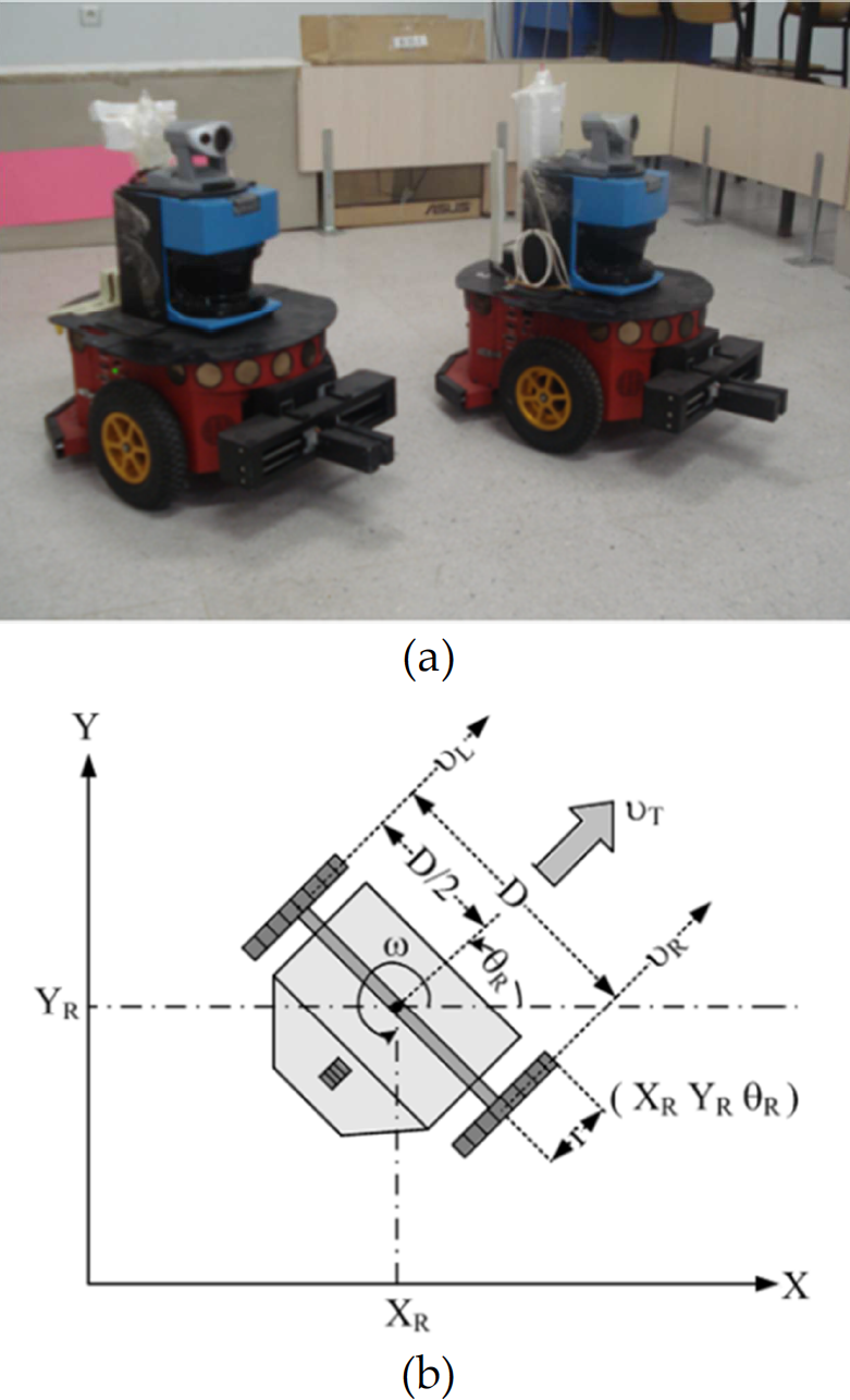
Mobile Robot Platform: (a) Pioneer P3-DX mobile robots, (b) the WMR and its parameters

Figure 3.

A curvature trajectory

3.2 Trajectory Generation

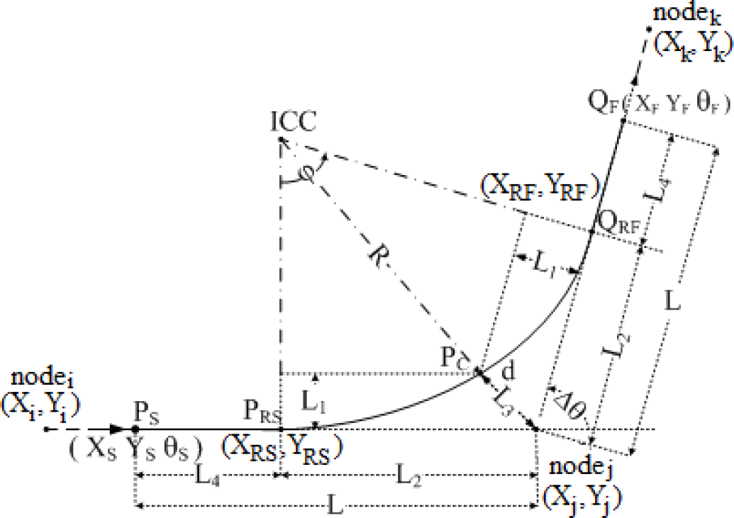
The path for the transportation of an object consists of critical nodes, as shown in Figure 4. These nodes can be connected using straight lines. However, due to the constraints of the robots, some parts of the path may cause the robots to make sharp turns. Additionally, the robots must slow down, orient themselves, and then accelerate. Thus, the object carried by the followers may fall. Therefore, the path should be smoothed by considering non-holonomic constraints.

Figure 4.

Some combinations of nodes on a path

Figure 5.

The symmetric curved path

The path defined by the straight lines can be transformed into a smooth trajectory, as observed in Figure 5 [24]. The trajectory may be considered in three sections, i.e., before, during and after the rotation. P_S = [X_S, Y_S, θ_S]^T is the initial point of the curve where the WMR may slow down and also wait if necessary. P_RS is the point where the WMR starts to follow a circular curve around the ICC with a radius of R. Q_RF is the point where the robot finishes its rotation, and Q_F=[X_F, Y_F, θ_F]^T is the final point where the WMR completes its tracking on the curved trajectory.

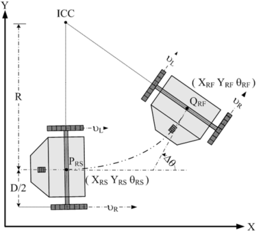
When the WMR is moving from P_RS to Q_RF, the difference between the initial and the final orientation of the robot is ∆θ and is expressed as follows:

$$\mathrm{\Delta }\theta ={\theta }_F-{\theta }_S$$

(4)

Because there are constraints imposed by obstacles, the bound of path-deviation L₁ from the corner at node_j is defined as follows:

$$\begin{array}{l}{L}_1=L_3\cos (\mathrm{\Delta }\theta /2)\\ L_2=R\tan (\mathrm{\Delta }\theta /2)\\ L_3=R\left[\frac{1}{\cos (\mathrm{\Delta }\theta /2)}-1\right]\\ L=L_2+L_4\end{array}$$

(5)

d is the total distance travelled by the WMR during the rotation with the rotation angle ϕ expressed in equation (6). During the rotation, the robot frequently updates its location and orientation, and controls the translational speed v_T, rotational speed ω, and heading angle θ_R.

$$\begin{array}{l}d={\displaystyle \underset{t_{P_{RS}}}{\overset{t_{Q_{RF}}}{\int }}\frac{{\upsilon }_L+{\upsilon }_R}{2}}dt\\ \phi =\frac{d}{R}\end{array}$$

(6)

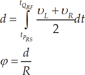
To generate a smooth path, the critical points P_S, P_RS, Q_RF, Q_F, and ICC should be determined by using the geometrical parameters shown in Figures 3 and 5.

The mathematical equations for the point ICC (ICC_x, ICC_y) are written as follows:

$$\begin{array}{l}{\theta }_s={\tan }^{-1}\left(\frac{Y_j-Y_i}{X_j-X_i}\right)\\ IC{C}_x=X_j+{\left(-1\right)}^{m}R\sin \left({\theta }_s\right)-L_2\cos \left({\theta }_s\right)\\ IC{C}_y=Y_j+{\left(-1\right)}^{m}R\cos \left({\theta }_s\right)-L_2\sin \left({\theta }_s\right)\end{array}$$

(7)

m indicates the turning direction of WMR. For m = 1 or m = 0, the WMR turns anti-clockwise or clockwise, respectively. The points P_S(X_S, Y_S), P_RS(X_RS, Y_RS), Q_RF(X_RF, Y_RF), and Q_F(X_F, Y_F) are defined as follows:

$$\begin{array}{l}{X}_S=X_j-L\cos ({\theta }_s)\\ Y_S=Y_j-L\sin ({\theta }_s)\end{array}$$

(8)

$$\begin{array}{l}{X}_{RS}=X_j-L_2\cos ({\theta }_s)\\ Y_{RS}=Y_j-L_2\sin ({\theta }_s)\end{array}$$

(9)

$$\begin{array}{l}{\theta }_F={\tan }^{-1}\left(\frac{{\begin{array}{c}Y\end{array}}_j-Y_k}{X_j-X_k}\right)\\ X_{RF}=X_j+L_2\cos ({\theta }_F)\\ Y_{RF}=Y_j+L_2\sin ({\theta }_F)\end{array}$$

(10)

$$\begin{array}{l}{X}_F=X_j+L\cos ({\theta }_F)\\ Y_F=Y_j+L\sin ({\theta }_F)\end{array}$$

(11)

3.3 Discrete-time Model

The discrete-time model of the robot is obtained from the integration of the equations (1) and (2) [27,28]. The discrete-time model is shown in Figure 6.

Figure 6.

Discrete-time model

At any instant, the centre of the VL [X_VL, Y_VL] changes due to its translational and rotational speed. The kinematic model of the VL assumes no slippage. Thus, its motion can be defined by the simple kinematics of rigid bodies. The posture of the VL can be estimated by integrating the equations given in equations (1) and (2). The integration is implemented by the following equations: (i) When ω_VL ≠ 0

$$\begin{array}{l}{x}_{\text{VL}}\left(k+1\right)=x_{VL}(k)+\frac{v_{VL}}{{\omega }_{VL}}\left[\sin \left({\theta }_{VL}\left(k+1\right)\right)-\sin \left({\theta }_{VL}\left(k\right)\right)\right]\\ y_{\text{VL}}\left(k+1\right)=y_{VL}(k)-\frac{v_{VL}}{{\omega }_{VL}}\left[\cos \left({\theta }_{VL}\left(k+1\right)\right)-\cos \left({\theta }_{VL}\left(k\right)\right)\right]\\ {\theta }_{VL}\left(k+1\right)={\theta }_{VL}(k)+{\omega }_{VL}{t}_s\end{array}$$

(12)

(ii) When ω_VL = 0

$$\begin{array}{l}{x}_{\text{VL}}\left(k+1\right)=x_{VL}(k)+v_{VL}{t}_s\cos \left({\theta }_{VL}\left(k\right)\right)\\ y_{\text{VL}}\left(k+1\right)=y_{VL}(k)+v_{VL}{t}_s\sin \left({\theta }_{VL}\left(k\right)\right)\\ {\theta }_{VL}\left(k+1\right)={\theta }_{VL}(k)\end{array}$$

(13)

where k denotes the sampling index and t _s is the sampling time. The posture vector [X_VL (k+1), Y_VL(k+1), θ_VL(k+1)]^t obtained from the equations (12) and (13) becomes the reference position and heading angle for the VL. Furthermore, the reference velocity vector [VL, VL]^t is determined by the desired translational and angular velocities specified by the user.

When the discrete-time model equations of VL are given by the equations (12) and (13), the equations for the followers are derived by using the coordinate transformation, given as follows:

$$\begin{array}{l}{x}_{Fi}\left(k+1\right)=x_{\text{VL}}\left(k+1\right)+d_i\cos \left({\alpha }_i+{\theta }_{VL}\left(k\right)\right)\\ y_{Fi}\left(k+1\right)=y_{\text{VL}}\left(k+1\right)+d_i\sin \left({\alpha }_i+{\theta }_{VL}\left(k\right)\right)\\ {\theta }_{Fi}\left(k+1\right)=\{\begin{array}{l}{\tan }^{-1}\left(\frac{y_{\text{Fi}}\left(k+1\right)-y_{\text{Fi}}(k)}{x_{\text{Fi}}\left(k+1\right)-x_{\text{Fi}}(k)}\right)if{\omega }_{VL}\ne 0\\ {\theta }_{VL}\left(k+1\right)if{\omega }_{VL}=0\end{array}\end{array}$$

(14)

where d _i and α _i (i = 1, 2, …, n) are the Euclidean distance and the angle between the i ^th follower and the VL, respectively.

The posture of the followers is expressed as [X _Fi (k + 1) Y _Fi (k + 1) θ _Fi (k + 1)] ^T . The desired linear and angular velocities of the i ^th follower, [v _Fi (k + 1) ω _Fi ] ^T , are different from the desired velocities of the VL. The velocities of the followers are found as follows:

$$\begin{array}{l}{\upsilon }_{x_{Fi}}\left(k+1\right)=\raisebox{1ex}{$[x_{Fi}\left(k+1\right)-x_{Fi}(k)]$}\!\left/ \!\raisebox{-1ex}{$t_s$}\right.\\ {\upsilon }_{y_{Fi}}(k+1)=\raisebox{1ex}{$[y_{Fi}\left(k+1\right)-y_{Fi}(k)]$}\!\left/ \!\raisebox{-1ex}{$t_s$}\right.\\ {\upsilon }_{Fi}(k+1)=\sqrt{{\upsilon }_{x_{Fi}}{}^2\left(k+1\right)+{\upsilon }_{y_{Fi}}{}^2\left(k+1\right)}\\ -{\omega }_{VL-\max }\le {\omega }_{Fi}\le {\omega }_{VL-\max }\end{array}$$

(15)

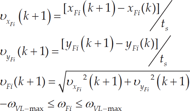
where ω_VL–max is the maximum angular velocity of VL.

In Section 4, these discrete-time models are used for trajectory tracking control.

3.4 Motion Constraints for WMR

To generate a feasible path for the VL, the kinematic constraints of the VL, $A(q)\dot{q}=0$ , should be considered. The Pfaffian constraint matrix for the WMR is expressed as follows:

$$\left[\begin{array}{ccc}-\sin \theta & \cos \theta & 0\end{array}\right]\left[\begin{array}{c}\dot{x}\\ \dot{y}\\ \dot{\theta }\end{array}\right]=0$$

(16)

Moreover, since the VL tracks a smooth trajectory considering kinematic constraints, a deviation between the orientation angles of i ^th follower and the VL is generated. During the transportation, this deviation should be minimized to avoid dropping the object from the forks. The maximum absolute allowable deviation is specified by the user as θ _desired . The constraint is expressed as follows:

$$\left|{\theta }_{VL}\left(k+1\right)-{\theta }_{Fi}\left(k+1\right)\right|\le {\theta }_{desired}$$

(17)

Followers may carry the object without dropping it since the constraint in equation (17) is considered to generate the trajectory. Using the equations (12), (13), and (14) considering the equation (17), a feasible path for the VL is generated, and the deviation angle stays within the range [−θ _desired , θ _desired ].

4. Robot Control Scheme

In the proposed system, the followers generate their own paths according to the VL. In fact, the reference postures of the followers are obtained by using the coordinate transformation of the VL's posture. During the transportation, the followers track its reference posture and velocities. Each follower uses a tracking controller. This section discusses two types of tracking controller: asymptotically stable tracking control [20] and sliding-mode control [21]. These controllers are designed using Lyapunov stability theory and achieve zero tracking error. Figure 7 shows the common block diagram of the tracking controllers. This diagram is composed of an error block, a control rule, a velocity limiter, and the robot's kinematic model.

Figure 7.

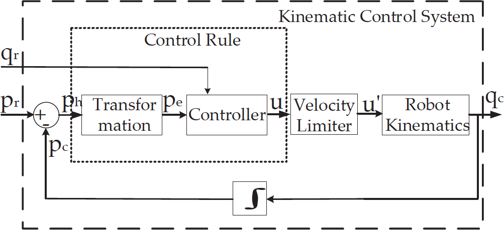
Block diagram of the tracking control system

Figure 8.

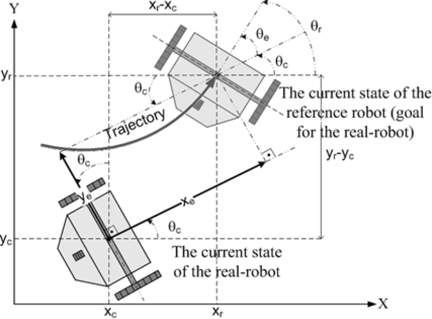
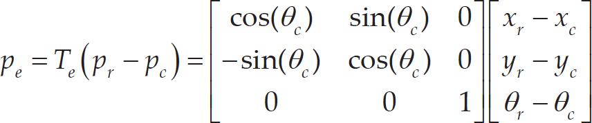
Error components

p _r = [ x _r y _r θ _r ] ^T and q _r = [ v _r ω _r ] ^T are inputs for the controller and indicate the reference posture and velocities, respectively. These inputs are obtained from the discrete-time models for the given path of the followers and the VL. u is the velocity vector including linear and angular velocities which is the output of the control rule, and u' is the output of the velocity limiter. Using the robot kinematics, the output of the tracking control system is the velocity vector q _c = [ v _c ω _c ] ^T which indicates the current linear and angular velocities of the robot. The current posture of the WMR, p _c = [ x y _c θ _c ] ^T , is obtained by integrating q _c . p _h = [ x _h y _h θ _h ] ^T is the posture error, given as follows:

$$p_h=p_r-p_c$$

(18)

For tracking control, p _h needs to be transformed to the robot's local coordinate axis. Thus, the posture error p _e = [ x _e y _e θ _e ] ^T is obtained. T _e is the transformation matrix as given in equation (19) to transform p _h to p _e .

$$T_e=\left[\begin{array}{ccc}\cos ({\theta }_c)& \sin ({\theta }_c)& 0\\ -\sin ({\theta }_c)& \cos ({\theta }_c)& 0\\ 0& 0& 1\end{array}\right]$$

(19)

For each follower, the posture error is calculated as the difference between the reference and the current posture of the followers according to the followers' local coordinate axis. The posture error is given by equation (20) as shown in Figure 8.

$$p_e=T_e\left(p_r-p_c\right)=\left[\begin{array}{ccc}\cos ({\theta }_c)& \sin ({\theta }_c)& 0\\ -\sin ({\theta }_c)& \cos ({\theta }_c)& 0\\ 0& 0& 1\end{array}\right]\left[\begin{array}{c}{x}_r-x_c\\ y_r-y_c\\ {\theta }_r-{\theta }_c\end{array}\right]$$

(20)

The derivative of the posture error, i.e., ${\dot{p}}_e={[{\dot{x}}_e,{\dot{y}}_e,{\dot{\theta }}_e]}^t$ , is obtained as follows [20]:

$${\dot{p}}_e=\left[\begin{array}{c}{\dot{x}}_e\\ {\dot{y}}_e\\ {\dot{\theta }}_e\end{array}\right]=\left[\begin{array}{c}{\omega }_c{y}_e-v_c+v_r\cos ({\theta }_e)\\ -{\omega }_c{x}_e+v_r\sin ({\theta }_e)\\ {\omega }_r-{\omega }_c\end{array}\right]$$

(21)

4.1 Asymptotically Stable Tracking Control

The control rule part, i.e., steering (velocity) controller, is obtained by feed-forward and feed-back actions. The structure of the control rule part is shown in Figure 9.

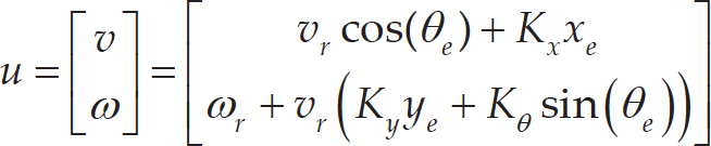
The feed-forward part of the output vector is illustrated as u _ff and the feed-back part of the output vector is presented as u _fb . The output of the control rule, i.e., u, is given in equation (22).

$$u=u_{ff}+u_{fb}$$

(22)

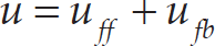
The feed-forward part provides necessary inputs to the robot in order to track the trajectory. A matrix, A, is defined for the feed-forward part as given in equation (23).

$$A=\left[\begin{array}{cc}\cos ({\theta }_e)& 0\\ 0& 1\end{array}\right]$$

(23)

Figure 9.

Inner block diagram of the control rule

The output of the feed-forward part, i.e., u _f = [v _ff ω _ff ] ^T , is obtained by using the matrix A and the reference velocity vector q _r = [v _r ω _r ] ^T as given in equation (24).

$$u_{ff}=A.q_r=\left[\begin{array}{cc}\cos ({\theta }_e)& 0\\ 0& 1\end{array}\right]\left[\begin{array}{c}{v}_r\\ {\omega }_r\end{array}\right]=\left[\begin{array}{c}{v}_r\cos ({\theta }_e)\\ {\omega }_r\end{array}\right]$$

(24)

The feed-back part includes gain, gain scheduling and natural frequency generator. It provides necessary inputs by using the posture error and the reference. The gain part includes K _x , K_θ and K_θ such that these parameters are positive constant and can be found by trial and error. The gain matrix, K, is defined as in equation (25):

$$K=\left[\begin{array}{ccc}{K}_x& 0& 0\\ 0& K_y& K_{\theta }\end{array}\right]$$

(25)

A matrix, B, is defined for the feed-back part as given in equation (26):

$$B=\left[\begin{array}{c}{x}_e\\ v_r{y}_e\\ v_r\sin ({\theta }_e)\end{array}\right]$$

(26)

The output of the feed-back part, i.e., u _fb = [v _fb ω _fb ] ^T , is obtained by using the matrix B and the gain matrix K, as given in equation (27):

$$u_{fb}=K.B=\left[\begin{array}{c}{K}_x{x}_e\\ v_r\left(K_y{y}_e+K_{\theta }\sin \left({\theta }_e\right)\right)\end{array}\right]$$

(27)

Using equations (24) and (27) in (22), equation (28) is obtained as follows:

$$u=\left[\begin{array}{c}v\\ \omega \end{array}\right]=\left[\begin{array}{c}{v}_r\cos ({\theta }_e)+K_x{x}_e\\ {\omega }_r+v_r\left(K_y{y}_e+K_{\theta }\sin \left({\theta }_e\right)\right)\end{array}\right]$$

(28)

Using equation (28) in equation (21) where the perfect velocity is considered $v\equiv v_c$ and $\omega \equiv {\omega }_c$ ), the derivative of the posture error, ${\dot{p}}_e={[{\dot{x}}_e,{\dot{y}}_e,{\dot{\theta }}_e]}^t$ , for asymptotically stable tracking control is expressed as in equation (29) and its stability is proven by using a Lyapunov function as given in [20].

$${\dot{p}}_e=\left[\begin{array}{c}[{\omega }_r+v_r(K_y{y}_e+K_{\theta }\sin ({\theta }_e))]y_e-K_x{x}_e\\ -[{\omega }_r+v_r(K_y{y}_e+K_{\theta }\sin ({\theta }_e))]x_e+v_r\sin ({\theta }_e)\\ -v_r(K_y{y}_e+K_{\theta }\sin ({\theta }_e))\end{array}\right]$$

(29)

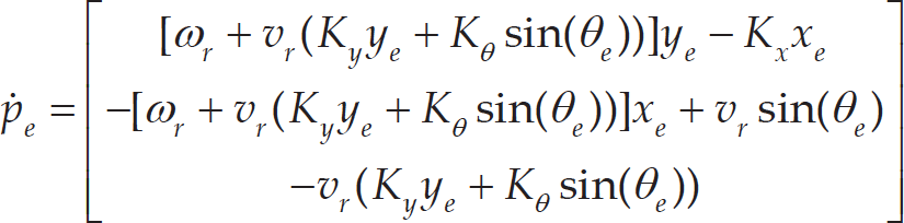
Using the linearization of ${\dot{p}}_e(t,e)=C(t)p_e$ around the equilibrium point p_e = [0 0 0] ^T , where C(t) is a Jacobian matrix, the K _y and K_θ gain parameters depend on damping factor, ζ, and natural frequency, ω _n , and are obtained as follows:

$$\begin{array}{l}{K}_y={\left(\frac{{\omega }_n}{v_r}\right)}^2\\ K_{\theta }=\frac{2\zeta {\omega }_n}{v_r}\end{array}$$

(30)

The system is stable for the positive gain parameters K _x , K _y and K_θ. The appropriate gain parameters should be found to ensure that the WMR has no oscillation and no slow response to the system as it tracks its trajectory. K _x , K _y and K_θ of the state feedback can be found by trial and error. In this study, some experiments are conducted to determine these values using a translational speed of the WMR between 50 and 400 mm/seconds. In these experiments, ζ is 1, ω is 4θ/seconds, and K _x is 1000. These values are kept constant. Thus, a seventh-order function of ω _n that depends on the WMR's translational speed is found. By using the function of ω _n and equation (30), K _y and K_θ are determined such that a gain schedule is realized. The function is as follows:

$${\omega }_{\mathrm{n}}\left(\mathrm{v}\right){\text{ = p}}_1{\mathrm{v}}^7+{\mathrm{p}}_2{\mathrm{v}}^6+{\mathrm{p}}_3{\mathrm{v}}^5{\text{+p}}_4{\mathrm{v}}^4{\text{+p}}_5{\mathrm{v}}^3{\text{+p}}_6{\mathrm{v}}^2{\text{+p}}_7{\text{v+p}}_8$$

(31)

where

$$\begin{array}{l}{\mathrm{p}}_1\text{ = 9}{\text{.651e-017, p}}_2\text{ = -1}{\text{.448e-013, p}}_3\text{= 9}{\text{.149e-011, p}}_4\text{= -3.129e-008, }\\ {\mathrm{p}}_5\text{= 6}{\text{.147e-006, p}}_6\text{ = -0}{\text{.0006744, p}}_7\text{ = 0}{\text{.03853, p}}_8\text{ = -0.4296}\end{array}$$

4.2 Sliding-mode tracking control

The expression of the control rule is given by

$$\left[\begin{array}{c}v(e,q,q_r,s)\\ \omega (e,q,q_r,s)\end{array}\right]=\left[\begin{array}{c}{y}_e\omega +v_r\cos ({\theta }_e)+k_{1}sat(s_1)\\ {\omega }_r+[\frac{y_e}{1+{(v_r{y}_e)}^2}]{\dot{v}}_r+[\frac{v_r}{1+{(v_r{y}_e)}^2}]v_r\sin ({\theta }_e)+k_{2}sat(s_2)\end{array}\right]$$

(32)

where s is the function of switching surface in the sliding mode expressed in equation (33); q = [v ω] ^T is the velocity vector of the WMR, where v is the linear velocity and ω is the rotational velocity; s is the reaching rule by replacing switching function with a saturation function; and k ₁ and k ₂ are the positive gain parameters, set to 120 in the experiments.

$$\begin{array}{l}s=\left[\begin{array}{c}{s}_1\\ s_2\end{array}\right]=\left[\begin{array}{c}{x}_e\\ {\theta }_e+\arctan (v_r{y}_e)\end{array}\right]\\ \dot{s}=-ksat(s)\end{array}$$

(33)

The stability of the control rule is proven using a Tyapunov function given in [21].

5. Experiments

The proposed cooperative transportation system for multiple autonomous non-holonomic mobile robots is coded in C++ and tested using P3-DX robots both in a MobileSim simulation environment and in real-world applications ¹ .

The P3-DX robot has an on-board P3-800 computer with Linux OS. The sensors on the robot include a SICK LMS laser range finder, a ring of 16 ultrasonic sensors, a camera, and a compass. A wireless network is supplied for communication among the robots and computers. The P3-DX robot has a 2-DOF gripper to grasp and carry objects. The platform has a sturdy aluminium body, balanced drive system (two-wheel differential with casters), reversible DC motors, motor-control and drive electronics, high-resolution motion encoders, and battery power, which are all managed by an on-board microcontroller and mobile-robot server software.

In the experiments, a 9000 mm × 9000 mm environment was used in the simulations, and a 7260 mm × 6655 mm environment in the real-world applications. The trajectories were generated for the VL by using equations (5) to (16). The trajectories passed over the nodes as shown in Table 1.

Table 1.

Nodes of the generated trajectories for the virtual leader

Nodes	Coordinates in Simulations		Coordinates in Real-world Applications
	X (mm)	Y (mm)	X (mm)	Y (mm)
Node 1	600	600	1000	1000
Node 2	3700	600	4000	1000
Node 3	3700	5600	4000	7000
Node 4	6400	5600	8000	7000

To identify the location of the robots, an odometer is used in simulations. In the real-world applications, the software library ARNL ¹ is used. This library implements the Monte Carlo Localization Algorithm to accurately place the robot within a given map by using the information derived from a laser-range and robot odometer.

To synchronize the robots during the transportation, an inter-robot communication framework is used. The followers track the reference inputs discussed in previous sections to maintain the formation with the VL. The VL has a 50 mm/s translational speed and a 5 degrees/s rotational speed in both the experiments and applications. Additionally, the value of θ_desired is set to 20 degrees.

In the experiments, the centre of mass of the objects is predefined by using the geometry and sizes of the objects; this is straightforward since the geometry and sizes of the objects are known in advance. However, the centre of mass may be defined by using images captured by the cameras of robots or cameras mounted around the environment.

5.1 Simulations

In the simulations, five different combinations are considered to transport a rectangular object. Figure 10(a-e) shows two robots carrying an object over their heads in line (Type 1), two robots carrying an object over their heads in parallel (Type 2), three robots carrying an object on their forks in a formation of triangular shape (Type 3), four robots carrying an object on their forks in a formation of rectangular shape (Type 4), and five robots carrying an object on their forks in a formation of pentagonal shape (Type 5), respectively. The deviation angle between the object and the followers should remain small when using the forks. Some numerical results of the experiments are given in Figure 11.

Figure 10.

Snapshots from the simulations: (a) two robots carrying an object in line (Type 1); (b) two robots carrying an object in parallel (Type 2); (c) three robots carrying an object in a formation of triangular shape (Type 3); (d) four robots carrying an object in a formation of rectangular shape (Type 4); (e) five robots carrying an object in a formation of pentagonal shape (Type 5).

As shown in Figure 10, the centre of gravity of the object tracks the reference path. A 2-norm of the tracking error for the object and the relative orientation of the followers with respect to the object are given in Figure 11 as the Maximum Absolute Tracking Error (MATE) in metres and the Maximum Absolute Relative Orientation (MARO) in degrees, respectively. The experiments are performed to analyse the results for the tracking controllers discussed previously and the different translational speeds of the VL to verify the effectiveness of the proposed system.

As observed in Figure 11, the sliding-mode controller provides better performance than the asymptotically stable tracking controller in the simulations in terms of MATE. If the upper limit of the MATE is set to 0.05 m, the tracking errors remain within a reasonable tolerance up to speeds of 0.2 m/s. Over 0.2 m/s, the MATE exceeds the tolerance. At this point, the tracking controller might be changed, or, using a mechanism, the upper limit of the MATE might be expanded. However, especially over 0.2 m/s, the asymptotically stable tracking controller performs better than the sliding-mode controller in terms of the MARO. Up to 0.2 m/s, the MARO are kept in the range [0, θ_desired].

Moreover, from Figure 11, it can be observed that increasing the translational speed of the VL makes the MATE of the object or the deviation of the object's centre from the reference path and the MARO increase. Up to 0.2 m/s, two types of kinematic tracking controller keep the MATE and MARO within a reasonable tolerance. Over 0.2 m/s, the MATE and the MARO might be exceeded such that a new motion planning including the dynamic properties of robots and a new tracking controller including dynamics parameters of robots should be used unless the upper limit of MATE and the value of θ_desired increase.

Figure 11.

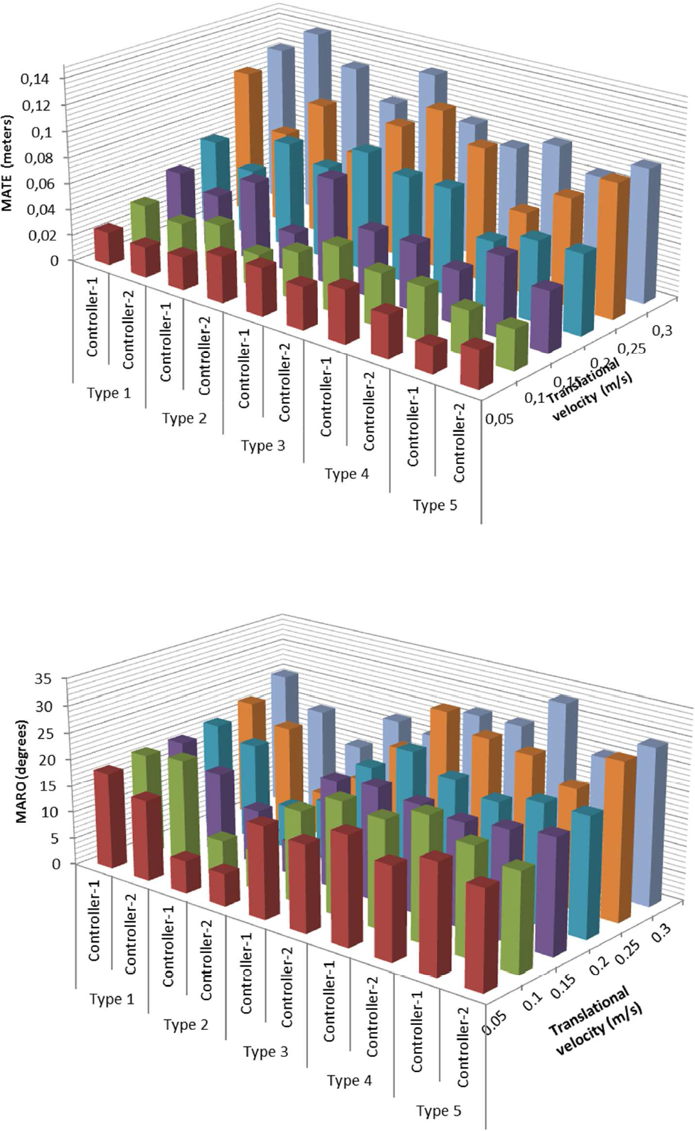
Test results of various setups for cooperative transportation. Type 1: two robots carrying an object in line; Type 2: two robots carrying an object in parallel; Type 3: three robots carry an object in a formation of triangular shape; Type 4: four robots carrying an object in a formation of rectangular shape; Type 5: five robots carrying an object in a formation of pentagonal shape; Controller 1: Asymptotically Stable Tracking Controller; Controller 2: Sliding-Mode Tracking Controller.

5.2 Real-world Applications

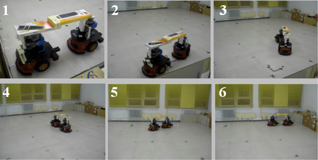
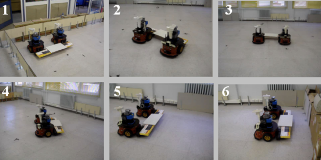
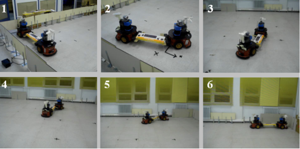
In the real-world applications, three Pioneer P3-DX mobile robots are used to transport an object in three different configurations. In the first two applications, two robots carry the object over their heads in line and in parallel, as seen in Figures 13 and 15, respectively. In the second two applications, two robots carry the object on their forks in line and in parallel, as seen in Figures 17 and 19, respectively. In the last application, three robots carry the object cooperatively on their forks, as seen in Figure 23. In the forklift case, it is noted that one of the followers moves backwards in contrast to the other followers. Videos of these applications are recorded in the Artificial Intelligence & Robotics Laboratory and can be found at the link in the footnote ² . Interested researchers can find pre-studies in [25–26].

5.2.1 Carrying the Object over the Robots' Heads

In these real applications, two robots carry an object over their heads in two different formations. The rectangular object is attached to the robots using an attachment mechanism, and transported over them. In the attachment, a T-shaped mechanism with a pin connection at the top is used to connect the object to the robots as seen in Figure 12.

Figure 12.

The handling mechanism: (a) schematic view of the handling mechanism, (b) the pallet as a transported object

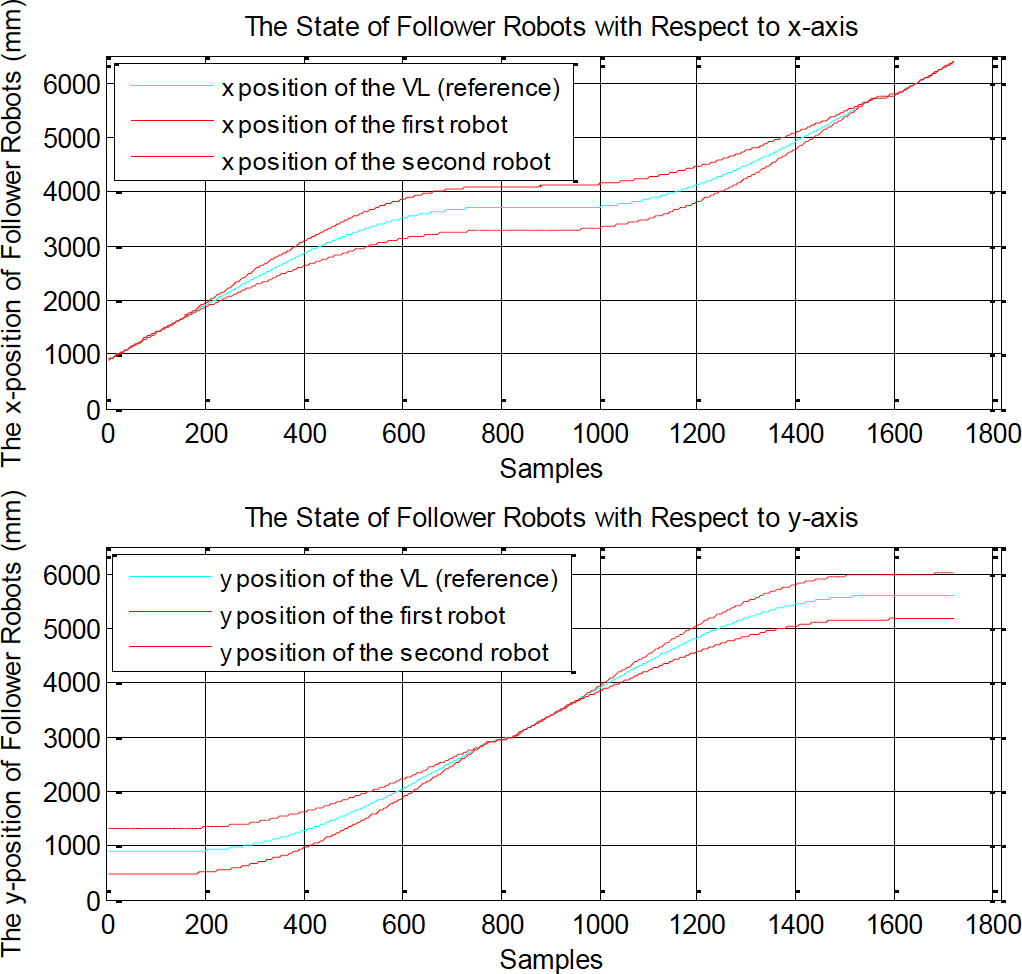
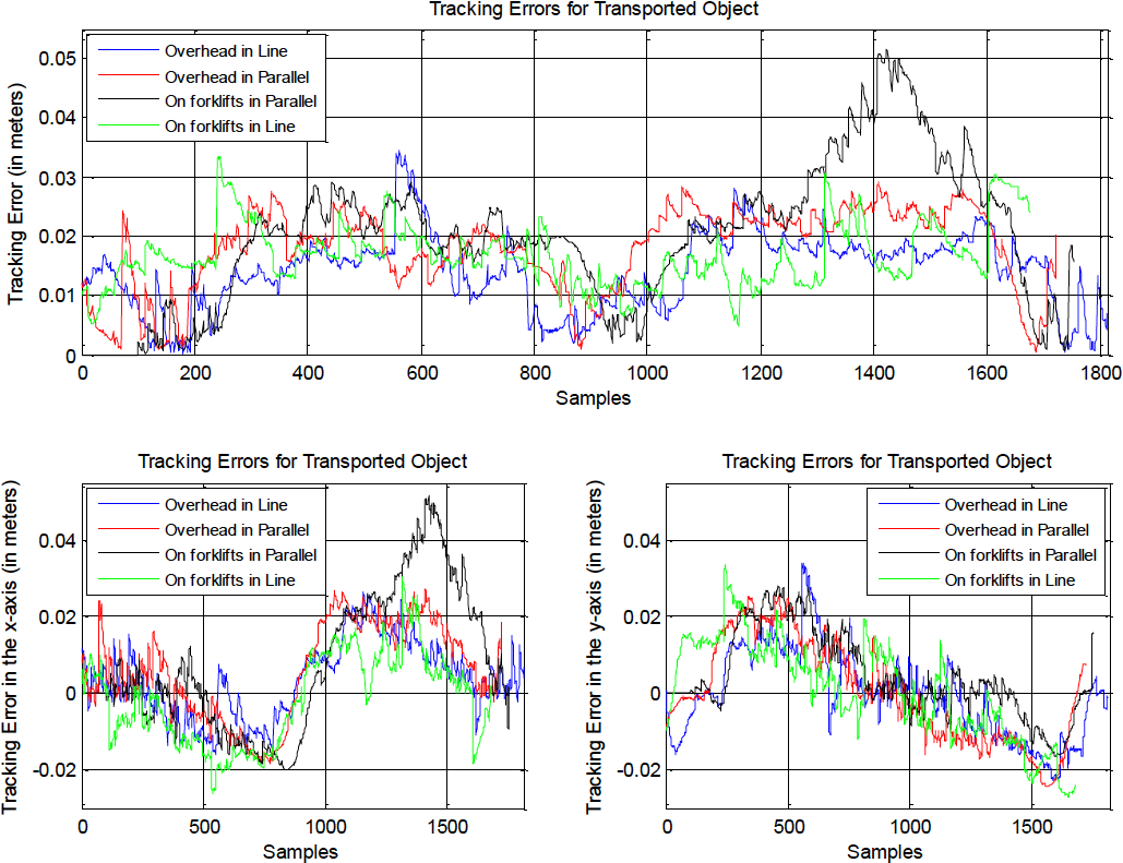
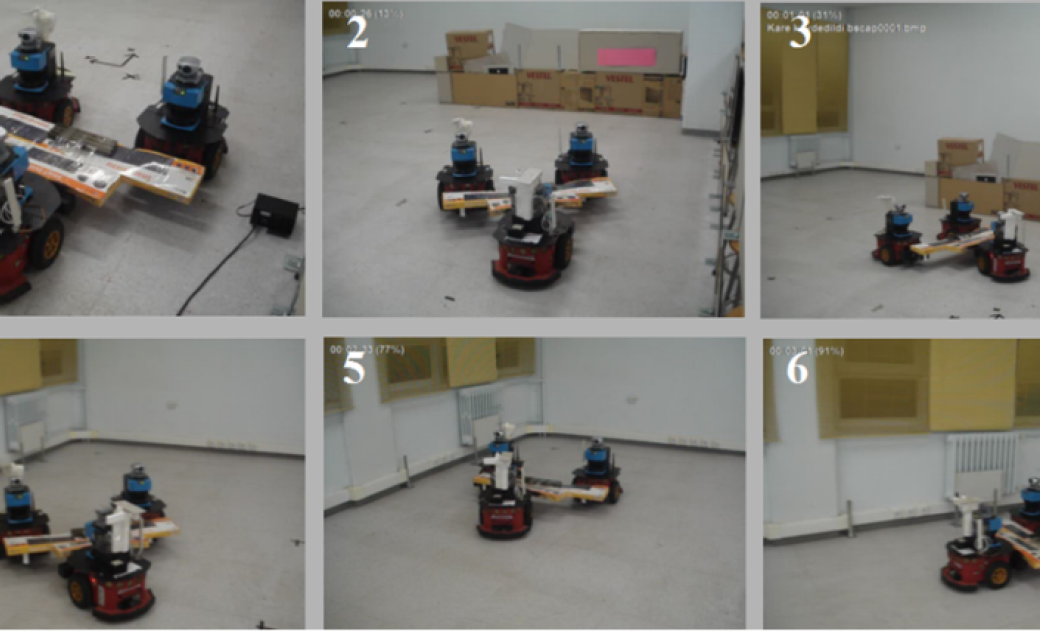
Figure 13 shows snapshots of the real-world application of the transportation system ³ . The follower robot's states in terms of x and y positions are illustrated in Figure 14, and the tracking error and the relative orientation angles are given in Figures 21 and 22. The formation type is two robots in line. The tracking errors of the transported object in the x- and y-directions are smaller than 35 mm. The relative orientation of the followers with respect to the object is less than 20 degrees. It is obvious that this angle is in the range of [−θ_desired, θ_desired].

In Figure 15, there are snapshots of the real-world application of the transportation system ⁴ . The follower robot's states in terms of x and y positions are illustrated in Figure 16, and the tracking error and the relative orientation angles are given in Figures 21 and 22. The formation type is two robots in parallel. The errors are smaller than 30 mm. As shown in Figure 22, the orientation angle is less than 6 degrees. The follower whose trajectory has a smaller radius than the other follower tracks its path slowly compared to the other follower while they are tracking their trajectories.

Figure 13.

Snapshot of a real-world application (two robots are carrying an object over head in a line form)

Figure 14.

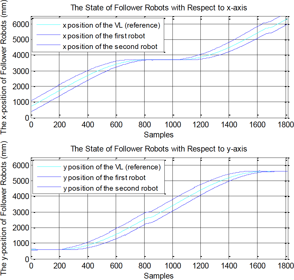
Robot states in terms of x and y positions (two robots carrying an object over their heads in line)

5.2.2 Carrying the Object on Forklifts of Robots

Three real applications are performed to carry an object on the forklifts of the robots. In the first application, two robots carry the object in a parallel formation as seen in Figure 17. In the second application, two robots carry the object in line as seen in Figure 19. In the last application, three robots carry the object in a triangular formation as seen in Figure 23. The rectangular object is placed on the forks of the robots and transported.

Figure 15.

Snapshot of a real-world application (two robots are carrying an object over their heads in parallel)

Figure 16.

Robot states in terms of x and y positions (two robots carrying an object over their heads in parallel)

Figure 17 shows snapshots of the real-world application of the transportation system ⁵ Two_robots_overhead_in_lme.wmv. The follower robot's states in terms of x and y positions are illustrated in Figure 18, and the tracking error and the relative orientation angles are given in Figures 21 and 22. The formation type is two robots in parallel. The tracking errors of the transported object in the x- and y-directions are smaller than 50 mm. The relative orientation of the followers with respect to the object is less than 5 degrees. It is obvious that this angle is in the range [θ_desired, θ_desired]. The follower whose trajectory has a smaller radius tracks its path slowly compared to the other follower while they are tracking their trajectories.

Figure 19 shows snapshots of the real-world application of the transportation system ⁶ . The follower robot's states in terms of x and y positions are illustrated in Figure 20, and the tracking error and the relative orientation angles are given in Figures 21 and 22. The formation type is two robots in line. It is noted that one of the followers has a reverse direction motion, unlike the other. The tracking errors are smaller than 35 mm. The orientation angle is less than 20 degrees. The follower that goes forwards tracks its trajectory forwards, and the follower that goes backwards tracks its trajectory backwards.

Figure 17.

Snapshot of a real-world application (two robots are carrying an object on forks in parallel)

Figure 18.

Robot states in terms of x and y positions (two robots carrying an object on forks in parallel)

Figure 19.

Snapshot of a real-world application (two robots carrying an object on forks in line)

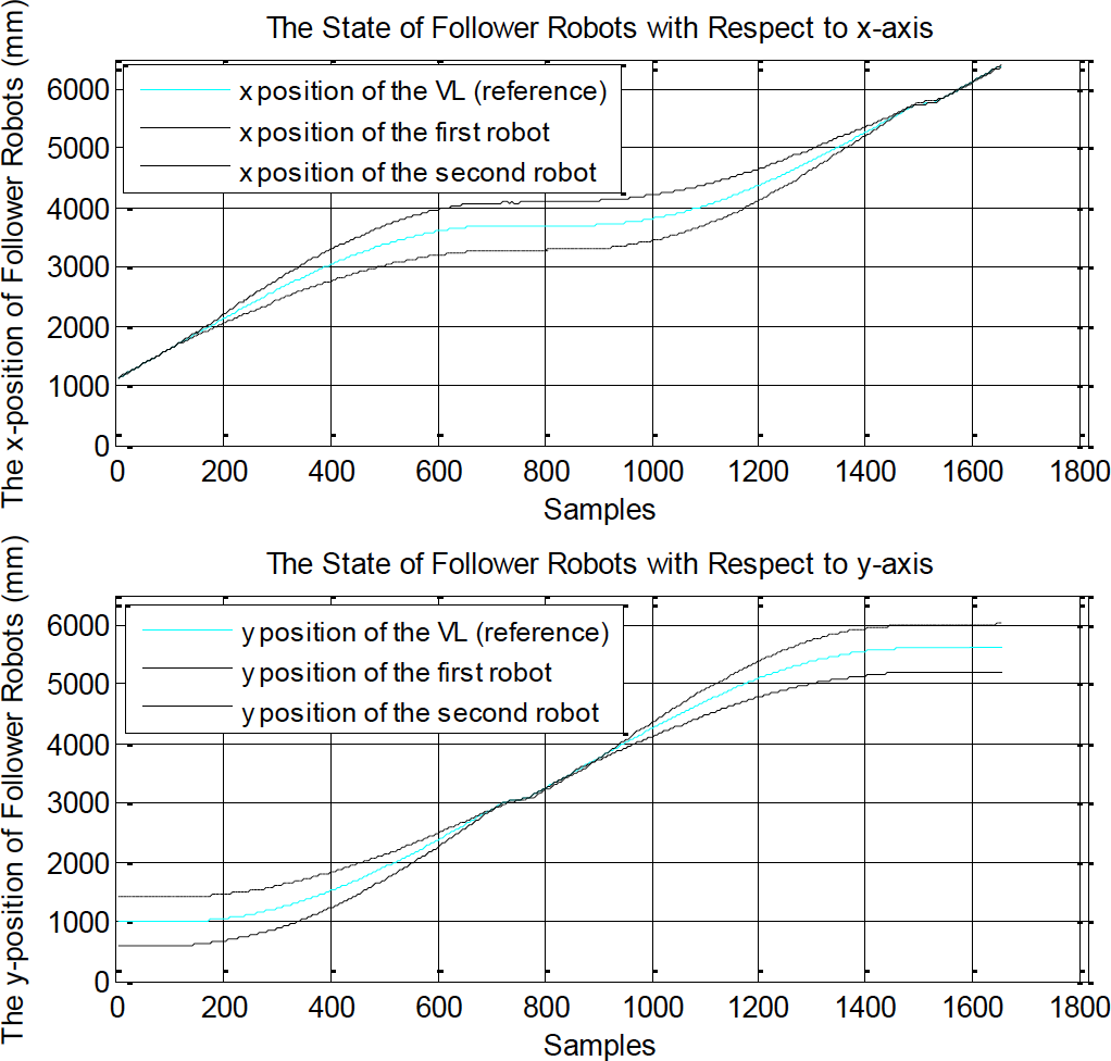
Figure 23 shows snapshots of the real-world application of the transportation system ⁷ . The formation type is three robots in a triangular formation. It is noted that two of the followers have a reverse direction motion, unlike the other follower. The follower that goes forwards tracks its trajectory in the forward direction and the other followers that go backwards track their trajectory in the backward direction. The errors are smaller than 30 mm. The relative orientation of the followers with respect to the object is almost 20 degrees; however, the robots maintain to carry the object over their forks even if the angle between the first follower and the object exceeds the value of θ_desired, i.e. 20 degrees. This overshoot may appear as robots rotate. Robot states in terms of x and y positions are illustrated in Figure 24, and results of this application are given in Figures 25 and 26.

Figure 20.

Robot states in terms of x and y positions (two robots carrying an object on forks in line)

Figure 21.

Tracking errors (in metres) for applications performed by two robots

Figure 22.

Relative orientation angle of followers with respect to the object (in degrees) for applications performed by two robots

Figure 23.

Snapshot of a real-world application (three robots carrying an object on forks)

Figure 24.

Robot states in terms of x and y positions (three robots carrying an object on forks)

Figure 25.

Tracking errors (in metres) for the application performed by three robots

6. Conclusions

The paper presents a formation-based cooperative transportation system comprising a group of non-holonomic mobile robots. Multiple robots are used to carry a large/heavy object, which a single robot is unable to do. The object is considered to be a robot as well (leader of the formation), and the movement trajectory from the origin to the desired destination point is computed. Initially, the followers communicate with each other for synchronization purposes; then, communication with each other or with a supervisor is not required in this system. Once the robots are synchronized, they behave in a distributed manner. A reference trajectory is generated for the virtual leader, and each follower robot generates its trajectory to satisfy the formation constraints. Two types of tracking controllers designed using Tyapunov stability theory are used by each follower robot. The performances of these controllers are compared. The robots carrying the object track their trajectories to maintain the formation with respect to the leader. Furthermore, to transport the single object cooperatively, the maximum or minimum number of followers depends on the weight, size and grasping points of the object. The shape of the formation also affects the number of followers.

The experiments with two, three, four and five robots carrying an object show that the proposed solution for cooperative transportation is quite effective. The errors from the ideal trajectory are within a reasonable tolerance. The results of simulations and real-world applications show that the proposed method effectively allows an object to be carried by multiple robots.

Future study will include applications of cooperative transportation both in real-world applications and simulations for different transportation tasks and numbers of robots.

Figure 26.

Relative orientation angle of followers with respect to the object (in degrees) for the application performed by three robots