
Abstract
Continuum robots exhibit great potential in a number of challenging applications where traditional rigid link robots pose certain limitations, e.g., working in unstructured environments. In order to enable the usage of continuum robots in safety-critical applications, such as surgery and nuclear decontamination, it is extremely important to ensure a safe path for the robot's movement. Existing algorithms for continuum robot path planning have certain limitations that need to be addressed. These include the fact that none of the algorithms provide safety assurance parameters and control for path planning. They are computationally expensive, applicable to a specific type of continuum robots, and mostly they do not incorporate design and kinematics constraints. In this paper, we propose a points-based path planning (PoPP) algorithm for continuum robots that computes the path by imposing safety constraints and improves upon the limitations of existing approaches. In the algorithm, we exploit the constant curvature-bending property of continuum robots in their path planning process. The algorithm is computationally efficient and provides a good tradeoff between accuracy and efficiency that can be implemented to enable the safety-critical application of continuum robots. This algorithm also provides information regarding path volume and flexibility in movement. Simulation results confirm that the algorithm possesses promising potential for all types of continuum robots (following the constant curvature-bending property). We believe that this effectively balances the desired safety and efficiency requirements.
Introduction
Robot designers have numerous design options when designing their machines. With time, the number of such design options continues to increase and/or be refined based upon technological advancements, inspiration from nature, and the designer's own imagination [1]. A number of different types of traditional rigid link robots have been proposed in the past. The design of these traditional robots is based upon a human arm-inspired mechanism, which consists of serially arranged rigid links or a joints-based architecture. Such traditional rigid link robots work fine in applications in which the environment is predefined and well-structured, but they have limitations in unstructured and congested workspaces [2]. To overcome the limitations of traditional rigid link robots, a large amount of research in continuum robotics has been published recently [2]. Continuum robots do not have rigid links/joints but present continuous flexibility in their structure. Because of their continuously bending architecture, continuum robots can manoeuvre through an unstructured congested workspace and can overcome the limitations posed by traditional robots [2, 3, 4].
In the literature, different types of continuum robot designs have been proposed that can be categorized as tendon-based, continuously bending actuator-based, concentric tubes-based, steerable needle-based or variable stiffness-based continuum robots [1, 4, 5]. Irrespective of their underlying physical architecture, the common property of the approximately constant curvature-bending of the backbone is exhibited by all types of continuum robots [4, 5]. This property has been exploited by different researchers to propose different designs and kinematics models of continuum robots [4, 5]. They exhibit significant potential in many challenging applications where traditional rigid links/joints-based robots have certain limitations. Examples of such applications involve working in obstacle-filled environments and minimally invasive surgery. For a robot to move from a given start location to a goal, the robot has to follow a path. There are certain constraints that the robot needs to follow during path planning. These constraints are: goal seeking, obstacle avoidance, non-penetration, spot the shortest path and energy minimization of the robot. For traditional rigid link robots, many path planning algorithms exist which solve a certain range of problems [6, 7]. For continuum robots, because of their continuously bending architecture and kinematics constraints, path planning brings many challenges that need to be addressed. Safety assurance is extremely important for the approval and usage of continuum robots in safety-critical applications, such as surgery. ISO 9000 standard norms have been updated to comply with the constraints of medical systems in the European Community. These standards allow the placement of such devices (e.g., continuum robots) in the market and their use for surgical applications.
Various research groups have proposed different methodologies for the path planning of continuum robots. However, there are certain limitations with existing approaches that need to be addressed. M. Moll and L.E. Kavraki proposed minimal energy curves-based path planning algorithms for deformable objects [8, 9, 10]. They introduced a new adaptive parametrization method for the representation of curves or configurations. Based on parametrization, they proposed methods for computing minimal energy curves, i.e., Lagrangian dynamics, null space sampling and constrained optimization techniques. They also proposed an algorithm for finding the sequence of minimal energy configurations between the start and goal configurations. The proposed methodology does not incorporate the obstacle avoidance and kinematics constraints that continuum robots have. This methodology is computationally expensive and is based on continuous deformation for specific shape-based path planning.
R. Gayle et al. proposed a medical image processing-based path planning algorithm for continuum robots [11]. During path planning, the algorithm checks for possible collisions between the robot and obstacles at each step. A special overlap test (2.5D) is used for finding the splitting surface between the robot and obstacles. The proposed algorithm does not incorporate the kinematics and design constraints of continuum robots. The algorithm is computationally expensive and uses a GPU-based collision detection algorithm. This may result in limited accuracy due to a lack of image-space resolution. In addition, the algorithm does not provide safety measures and control for safety-critical applications. E. S. Conkur and R. Gurbuz proposed a path planning algorithm for snake-like robots [12]. The algorithm consists of two steps, firstly it computes the smoothly curved path consisting of points from a given start to a goal point, and secondly the robot performs a serpentine motion on the previously computed path consisting of a number of points. The path trace from a given start point to a goal point is computed using the numerical potential field method (PFM). However, the proposed algorithm provides a discrete serial links-based path, and does not incorporate safety parameters. L. Lyons et al. proposed a motion planning algorithm for active cannulae-type continuum robots [13]. In the proposed algorithm, given the start and goal coordinates with obstacle information, the motion planning problem is formulated as a nonlinear constrained optimization problem. The PFM has been used for obstacle avoidance and for finding the optimal configuration of an active cannula. The limitation of the proposed methodology is that it is intended for use in image-guided procedures where the target and obstacles can be segmented from preoperative images. The methodology is robot-specific (limited to active cannulae), computationally expensive, and does not provide accommodation for safety parameters and control.
I. Godage et al. proposed a path planning algorithm for multisection continuum arms [14]. The algorithm was originally presented by Maciejewski et al. in [15] for the path planning of rigid link robots. This original algorithm was modified for continuum robots by incorporating a finite number of proximity sensors mounted along the length of the continuum robot to provide distal information. This information is used to find the repelling velocities of different sections of continuum robots, which are then used for goal seeking and obstacle avoidance. The proposed algorithm takes inputs from multiple sensors placed along the sections of the continuum robot, which might not be desirable for certain applications [1,16]. The algorithm also requires a points-based path trace as input. It is robot-specific, computationally expensive and does not provide safety parameters and control for safety-critical applications. C. Bergeles and P. Dupont proposed an algorithm for planning stable paths for concentric tube robots [17]. The rapidly-exploring random tree (RRT*) algorithm, presented by S. Karaman et al. in [18], is used for the path planning of the robot. For goal seeking, their algorithm navigates the robot through a sequence of locally stable configurations. Their work makes a good contribution to finding locally stable configurations for the path planning of active cannulae. However, the algorithm is robot-specific (limited to active cannulae), based on a variable curvature, computationally expensive, and does not incorporate safety parameters and control [17].
The main contribution of this paper is the proposed PoPP algorithm for continuum robots, which computes the locally optimal path by imposing safety constraints and improves upon the limitations that have been identified in existing approaches. The PoPP algorithm comprises two steps. Firstly, it computes the points-based path trace. Secondly, it finds the constant curvature (circular) curves-based continuous path using the points-based path trace as input. Both of these algorithms are internally used by the PoPP algorithm to generate a constant curvature curves-based continuous path for the continuum robot.
The Points-based Path Planning Algorithm
Continuum robots can interact and perform certain tasks in a workspace by using their tip/head as an end-effector. Hence, the tip/head is considered as a point of interest of continuum robots. Continuum robots emulate snake-like motion. The path planning of continuum robots in static environments is fairly simple because the rest of the body of the robot will most probably follow the track made by the head of the robot. By finding the track of the head of the continuum robot, we can find the path of the whole robot by traversing the head trace. Based on this idea, we propose algorithms to find the points-based path trace. The problem statement for the points-based path trace algorithm is: given start and goal points, find all the intermediate points that connect the start point and the goal point such that no intermediate point collides with any obstacle and the resulting path trace satisfies the imposed safety constraints.
The PoPP algorithm is divided into two steps: points-based path trace computation and constant curvature continuous path computation. For computing a points-based path trace, we propose two algorithms in Section 2.1 – one uses a sine method (SM) and the other uses the PFM. Both these approaches differ based upon their obstacle avoidance strategy. The SM exploits the information from the shortest distance vector to the obstacle, and then the vector to the goal point, while the PFM exploits the traditional PFM. Both approaches return a path trace connecting the start point and the goal point satisfying the constraints of obstacle avoidance as well as the safety parameters. For a continuum robot to follow a certain path, it needs to be continuous and the motion produced should be based on a constant curvature [4, 5]. This is so that the path satisfies the design and kinematics constraints of continuum robots. The points-based path trace returned by both approaches is discrete and does not satisfy the design and kinematics constraints for continuum robots. Hence, for this purpose, in Section 2.2, we propose a constant curvature curves-based continuous path planning algorithm. This algorithm takes the points-based trace of the path (resulting from the algorithms proposed in Section 2.1) as input and provides us with a continuous constant curvature curves-based path that satisfies the design and kinematics constraints of a continuum robot. The notation and symbols used in this paper are mostly defined locally in the algorithms; however, some of the globally-used nomenclature is defined in Table 1.
Nomenclature used in this paper
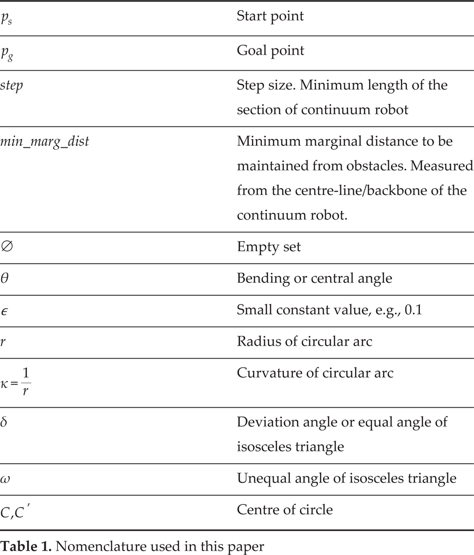
Nomenclature used in this paper
We propose two algorithms for computing a points-based path trace. Both algorithms take the start point, the goal point, the step size and the minimum marginal distance required from obstacles as input, and return the sequence of points connecting the start point and the goal point, such that none of the intermediate points collide with any obstacle and that it satisfies the safety parameters. Let us present each approach, one after another.
The Sine Method Algorithm
The basic idea of the sine method (SM) is explained in Algorithm 1. The algorithm first initializes the path with the start point ps and places the head pointer over start point ps. Next, we keep on iterating until the distance between the head and goal point pg is greater than or equal to the step. With each iteration, the head pointer is updated with the intermediate point. In the body of the iteration loop, we find the intermediate point pi at a distance step away from the head in the direction of pg. The intermediate point pi will be a shorter distance from the goal point than the head point, with a difference of step, and will be moving linearly towards the goal point pg. We then run the handleObstaclei() function (Algorithm 2) over the newly computed intermediate pointpi. The handleObstacle() function returns the obstacle-free intermediate point
In the Algorithm 1, the handleObstacle() function takes the head point, the intermediate point, the goal point and the minimum distance required from the obstacles as input, and returns the obstacle-free safe intermediate point as its output. The basic idea is explained in Algorithm 2. The algorithm first checks whether the intermediate point pi is not colliding with any obstacle and is away than min_marg_dist from the obstacle, i.e., the intermediate point is a safe point. If so, then return the same point pi as the output point. If it is colliding with or being influenced by the obstacle, then find the current angle (θ) of the intermediate pi, such that pi−1 is the centre of the circle and pi is a point on the circle. To avoid the obstacle, we either move clockwise or counterclockwise. Hence, to find the direction to avoid the obstacle (local optimal), we compute the vector
Differences between the SM and tangent bug algorithms

Differences between the SM and tangent bug algorithms
Without loss of generality, assume that we have a continuum robot with a section(s) with a diameter of 2mm and that we want to plan a path through a mathematically defined environment of 180mm × 180mm such that robot maintains a marginal distance of 3mm from the obstacles boundary. For the purpose of simulations, the obstacles' coordinates are known to the program; however, the algorithm takes the obstacles as unknown and finds the points-based path trace from the start to the goal points such that the path satisfies the imposed safety constraints. The algorithm has two safety parameters, i.e., the step size and the minimum marginal distance from the obstacles. The minimum marginal distance will be the sum of the radius of the continuum robot and the minimum distance to be maintained from the obstacles. For the above problem, the minimum marginal distance (min_marg_dist) will be passed as 1mm + 3mm=4mm. This is the minimum min_marg_dist value to be passed to the algorithm and the step size should be less than this value or else the robot may violate the safety constraints. For the above problem, if we pass the step size as 3.5mm and run the SM algorithm, then Figure 1 illustrates the resulting points-based path trace. If we decrease the step size value, then the resulting path becomes closer to the absolute path and reduces the path error. If we increase the step size value, then the resulting path behaves the other way around, i.e., it increase the path error. The other safety parameter, i.e., min_marg_dist, maintains the provided safety distance from the obstacle for the resulting points-based path trace.

Working of the SM for computing the points-based path trace in different environments
It is to be noted that there exist some apparent similarities between the SM algorithm and the tangent bug algorithm [21], e.g., the motion towards the goal and the boundary following behaviour. However, both are theoretically different from each other, as illustrated in Table 2. The SM algorithm works more efficiently in avoiding convex obstacles, does not require the computation of tangent points, and leaves the obstacle more efficiently, resulting in a shorter distance compared to the tangent bug algorithm.
The SM algorithm results in a path trace with fewer oscillations; however, it has certain limitations, e.g., it provides a local optimal path, poses limitations in environments with special convex obstacles, and is somewhat time-expensive around the obstacles boundary. To address these limitations posed by the SM, we present an alternative approach to determine the points-based path trace. This approach is based on the customization of the traditional PFM originally presented by O. Khatib [19]. In the PFM, the goal generates an attractive potential field while the obstacle generates a repulsive potential field. The path direction is computed by combining the two potential fields and following the force induced by the new, combined field to reach the goal by avoiding obstacles. The basic idea is explained in Algorithm 3.
Algorithm 3. first initializes the path with the start point ps and places the head pointer over the start point ps. Next, the algorithm keeps on iterating until the distance between the head and the goal point pg is greater than or equal to the step. With each iteration, the head pointer and path array will be updated with the intermediate path point. In the body of the iteration loop, we first find the attractive potential field vector
After computing the attractive and repulsive potential fields, we compute the total potential field
The Constant Curvature Curves-based Continuous Path Planning Algorithm
Continuum robots do not contain any rigid links or joints and consist of a continuously bending architecture [4]; hence, for a continuum robot to follow a particular path, the path needs to be continuous. Additionally, a common property of the approximately constant curvature-bending of the backbone is virtually exhibited by all types of continuum robots [4, 5]. Hence, the motion produced for the continuum manipulator should be a constant curvature (circular) curves-based path movement, such that the path satisfies the design and kinematics constraints of continuum robots. The path trace resulting from the approaches presented in Section 2.1 is discrete and does not satisfy the design and kinematics constraints of continuum robots. Moreover, as discussed, continuum robots cannot follow such a path because of their design and kinematics constraints. To compute the path that satisfies the design and kinematics constraints of continuum robots, we have proposed a path planning algorithm based on constant curvature curves. The algorithm takes the points-based path trace (resulting from the algorithms presented in Section 2.1) and the initial tangent/orientation vector as input, and provides a constant curvature moves-based continuous path as output. The resulting path now satisfies the design and kinematics constraints of continuum robots. The algorithm is based on fitting the constant curvature curves between path points by maintaining the continuity of the path. The curvature is defined as the degree to which the curves deviate from being a straight line. For a curve, the rate at which the tangent vector changes direction with respect to the arc length is called the “curvature” (κ) [20]. In circular curves, the rate of change of the tangent vector's direction is constant; hence, these are called “constant curvature curves”. The curvature is the reciprocal of the radius [3, 20]. Circles with a smaller curvature imply a larger radius, and vice versa. For a circle of radius r, the curvature κ can be computed as follows:

Next, we define the theoretical aspects of the constant curvature curves-based continuous path planning algorithm by exploiting it geometrically. For input, we take the path points shown in Figure 2. To fit the constant curvature curve between path points P1 and P2 (highlighted in Figure 2), we need the initial direction to maintain the continuity of the path. This initial direction can be maintained using the tangent vector at point P1 This vector will be the tangent on the previously fitted curve, e.g., between P0 and P1 at pointP1. The constant curvature curve fitted between path points P1 and P2 needs to maintain the continuity with the path. The tangent vector at point P1 on the previously fitted curve should guide this continuity and help us in pruning out all the other curves that do not satisfy the continuity constraints. Hence, we take point P1 such that it guides the tangent at point Pt as depicted in Figure 2. There are other methodologies to maintain the tangent [20], but we have used a points-driven tangent vector for maintaining continuity. This will also, later on, help in the selection of curves with the same curvature to satisfy the continuity constraint.

Fitting an isosceles triangle between points P1 and P2 to find the degree of curvature (θ)
The vector from
We exploit the properties of an isosceles triangle to fit the constant curvature continuous curve between path points P1 and P2. We find the bending angle or central angle (θ) of the curve to be fitted between P1 and P2. This angle is also referred as the “degree of curvature”. Using angle θ, we find the radius and hence the curvature of the curve using Equation (1). We fit the isosceles triangle such that one of the equal edges follows the tangent vector
The unequal angle (ω) of the isosceles triangle can be computed using ω = 180−2(δ). Based upon ω we can compute the degree of curvature using θ = 180ω. The angle θ can be directly computed from δ as follows:

The angle θ known as the bending angle or the central angle of the curve provides information for the circular curve between points P1 and P2. To find the curvature of the curve, we first need to find the radius of the curve to be fitted between P1 and P2. The radius (r) can be computed by exploiting the properties of the isosceles triangle CP1P2 and the right-angled triangle CPmP2, as demonstrated in Figure 3.

Computing the radius and the tangent vector at point P2.
To find the radius (r), we need to know the angle

In addition, the length of the edge PmP2 is equal to half of the Euclidean distance between points P1 and P2, i.e.,

Using Equations (2), (3) and (4), the radius (r) can be computed as follows:
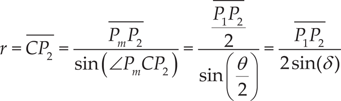
As such, the curvature (κ) can be computed using Equation 1. This value of κ represents the curvature of the circular curve to be fitted between points P1 and P2.
There are two possibilities for fitting the circular curve given the curvature/radius of the circle and the two end-points of the circular curve. One curve satisfies the continuity constraint, while the other does not. This has been pictorially demonstrated in Figure 4.

Two circular curves between points P1 and P2 based upon the radius/curvature
We have exploited the tangent vector
For finding the iso-edge-length

Using

Constant curvature curves-based continuous path for a continuum robot with a diameter of 2mm in a 18cm×18cm space
In this section, we compare our proposed algorithm with existing algorithms and analyse the novelties of our research work. The PoPP algorithm computed the path by imposing safety constraints and catered for the limitations of existing approaches. The algorithm has two safety parameters: the step size and the minimum marginal distance. The step size should be less than the minimum marginal distance so as to ensure that the continuum robot does not collide with an obstacle. If we set the step size as so small that it becomes negligible when compared to the minimum marginal distance, then the path becomes very close to the true path and the path error becomes negligible. There exists a good tradeoff between accuracy and efficiency. By decreasing the step size, the path error decreases as well, but it increases the running time of the algorithm. This works the other way around when we increase the step size. The second safety parameter – the minimum marginal distance – maintains the safety distance from obstacles. We proposed two algorithms for computing the points-based path trace, i.e., the SM algorithm and the PFM algorithm. The SM algorithm computes the path trace with fewer oscillations, better smoothness and fewer chances of getting stuck in the local minima. However, it provides the local optimal path, works efficiently for avoiding convex obstacles, needs improvements for avoiding special concave obstacles, and is somewhat time-expensive around the obstacles boundary. On the other hand, the PFM algorithm addresses the limitations of the SM algorithm, to some extent, but the path generated may have oscillations and may become stuck in the local minima. The PFM algorithm is faster compared to the SM algorithm, and enormous research has been carried out regarding its applications in traditional rigid link robots which can be incorporated for an efficient path trace. From Figure 6, we observed that the SM algorithm is slightly more time-consuming compared to the PFM algorithm.

Time complexities graph for points-based path trace algorithms (SM algorithm and potential field algorithm) and constant curvature curves-based continuous path planning (CC)
Comparison of PoPP with existing algorithms

Continuum robots consist of continuously bending architectures [4]; hence the path of continuum robots needs to be continuous. Furthermore, the backbones of all types of continuum robots can be visualized as a serially arranged, approximately constant, curvature curves-based configuration [4, 5]. Hence, the path moves should consist of constant curvature (circular) curves-based path moves such that the path satisfies the design and kinematics constraints of continuum robots. The points-based path trace resulting from the approaches presented in Section 2.1 (SM algorithm and PFM algorithm) is discrete and does not satisfy the design and kinematics constraints of continuum robots. This path trace is used by the constant curvature curves-based continuous path planning algorithm as input and computed the constant curvature curves-based continuous path for the continuum robots. From Figure 5, we can visualize that the path generated by the constant curvature curves-based continuous path planning algorithm is continuous and is based on constant curvature curves-based path moves. Hence, the resulting path satisfies the design and kinematics constraints of continuum robots. The smoothness and curvatures of the path depends upon the smoothness of the points-based path trace passed as input to the constant curvature curves-based continuous path planning algorithm. Fewer oscillations and curvature changes in the points-based path trace result in a smoother constant curvature curves-based continuous path. Figure 5 shows the configuration of an n-section continuum robot at different time slots, following the initial configuration t1 t2,…tn. For the path in Figure 5, n=56 (with 57 path points). Figure 7 shows the curvature variations of the path at different time slots. These curvature variations can be used for computing the volume of the path hose and dexterity for the robot's movement at a certain time slot. From Figure 6, we can observe the time complexity of the constant curvature curves-based continuous path planning algorithm (CC). We observed that the constant curvature curve fitting algorithm takes approximately 0.3 seconds for a path consisting of 1,000 path points. MATLAB 7.10 R2010a has been used with a 2.5 GHz PC processor for generating the simulations and computing the time complexities of the algorithms proposed in this paper.
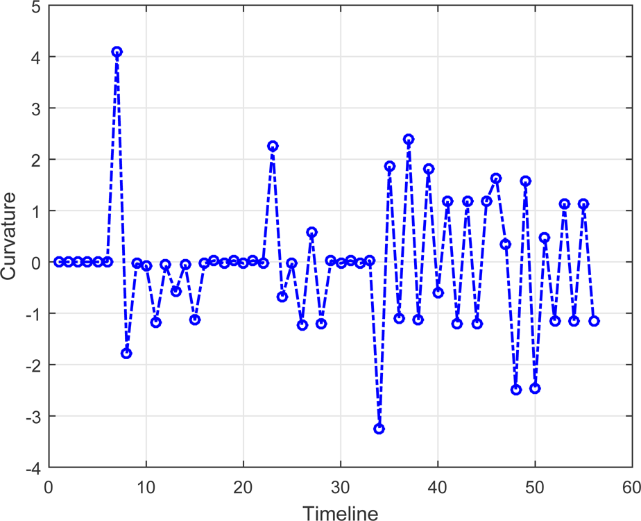
Curvature of the path at different time slots
The PoPP algorithm takes approximately 0.47 (0.3 + 0.17) seconds for computing a complete path consisting of 1,000 path points (Figure 6). The PoPP algorithm has been demonstrated to be more efficient compared to existing algorithms (see Table 3 for a comparison). This is because, firstly, it is points-driven and, secondly, it does not find the configurations of all the sections of the continuum robot for different time slots. Rather, the body of the continuum robot follows the path trace made by the head (first section) of the continuum robot. As such, the algorithm simply finds the configurations of the first/head section of the continuum robot, while the rest of the body follows the path trace of the head section in consecutive time slots. The 1,000 points-based path can be visualized as any number of sections of a continuum robot, ranging from 1–999, following the path in different time slots. Hence, the algorithm exhibits sound potential for applications with continuum robots with any number of sections to achieve the desired safety with speed. Additionally, the algorithm is applicable to all types of continuum robots satisfying the property of constant curvature-bending for their manipulators. This also addresses the limitations of existing algorithms for the path planning of continuum robots, which are applicable to specific types of continuum robots with a limited number of sections (mostly three) and which are computationally expensive (ranging from seconds to hours) with limited accuracy.
In this paper, we proposed a PoPP algorithm for continuum robots in two-dimensional environments. Existing algorithms for the path planning of continuum robots are robot-specific and do not provide safety measures, assurance or control. They are computationally expensive and mostly they do not incorporate design and kinematics constraints. Safety assurance is extremely important for the approval and usage of continuum robots in safety-critical applications. In the PoPP algorithm, we exploited the constant curvature backbone bending property of continuum robots, and provided a constant curvature curves-based continuous path satisfying the safety, design and kinematics constraints of continuum robots. The algorithm also addresses the limitations of existing algorithms for the path planning of continuum robots. We have confirmed that the algorithm also provides information about the volume of the path hose and flexibility of movement at different time slots. The algorithm exhibits promising potential for applications with all types of continuum robots-following the constant curvature backbone bending property – to achieve the desired safety with efficiency. In addition, the algorithm provides a good tradeoff between accuracy and efficiency that can be exploited for safety-critical applications of continuum robots, e.g., minimally-invasive surgeries. Future research is in progress to optimize the performance of the points-based path trace algorithms and the constant curvature continuous path planning algorithm.
Footnotes
5.
The authors would like to thank National University of Sciences and Technology (NUST), Islamabad, Pakistan for their support to complete this research project.