Sage Journals: Discover world-class research

Abstract

Jumping-height-and-distance (JHD) active adjustment capability is important for jumping robots to overcome different sizes of obstacle. This paper proposes a new structural-parameter-based JHD active adjustment approach for our previous jumping robot. First, the JHD adjustments, modifying the lengths of different legs of the robot, are modelled and simulated. Then, three mechanisms for leg-length adjustment are proposed and compared, and the screw-and-nut mechanism is selected. And for adjusting of different structural-parameters using this mechanism, the one with the best JHD adjusting performance and the lowest mechanical complexity is adopted. Thirdly, an obstacle-distance-and-height (ODH) detection method using only one infrared sensor is designed. Finally, the performances of the proposed methods are tested. Experimental results show that the jumping-height-and-distance adjustable ranges are 0.11 m and 0.96 m, respectively, which validates the effectiveness of the proposed JHD adjustment method.

Keywords

Jumping robot biologically inspired robot structural parameter jumping height and distance adjustment obstacle detection obstacle overcoming

1. Introduction

Jumping locomotion can help creatures in nature to traverse unstructured environments efficiently to hunt for food and escape from their natural enemies [1], especially for small insects such as locusts [2], froghoppers [3], and fleas [4]. Inspired by jumping animals, researchers have developed a great many jumping robots [5–8] for possible applications in planetary exploration [9], search and rescue [10], reconnaissance [11], mobile sensor networks [12], and so on.

Jumping-height-and-distance (JHD) adjustment capability is crucial for negotiating different heights of obstacles and different widths of ditches for jumping robots. However, few existing jumping robots have an active JHD adjustment function. The third generation of the JPL robot [13] is able to adjust its JHD by using a take-off-angle adjustment system. The SandFlea utilizes a leg under its body for JHD adjustment [11]. Our previous continuous-jumping robot [14–16], shown in Figure 1, is capable of adjusting its JHD actively by using a pole leg and an additional weight (AW) for adjusting its centre of mass (COM). However, this method has some disadvantages. Firstly, the heavy AW lowers the energy efficiency of the robot. Secondly, the JHD can only be adjusted from 88 cm to 93 cm and 20 cm to 60 cm, respectively. The adjustment ranges are larger only when the AW is heavier. Lastly, the location of the AW changes when the pole leg rotates on the front surface of the robot. The COM of the robot also changes to the left or right side, which leads to lateral shift of the robot during jumping locomotion.

Figure 1.

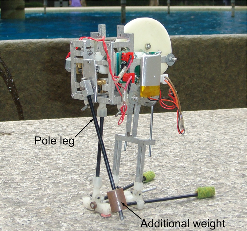
Our previous jumping robot, presented at IROS 2012, has jumping-height-and-distance active adjustment capability that uses a pole-leg and an additional weight for COM-position adjustment

Body structures of animals and insects can influence their locomotion performances. Steudel-Numbers et al. found that people with relatively longer lower limbs have lower locomotor costs during walking [17] and running [18]. Pontzer reported that effective limb length drives the scaling of locomotor cost for terrestrial animals [19].

In addition to studying the effects of body structures on animals’ locomotion performances, researchers have also begun to investigate the effects of structural parameters on locomotion performances of manmade machines. Structural parameters of articulated mechanisms can be optimized to improve performances of jumping robots. Lim et al. developed optimization algorithms to improve the performance of a biarticular-legged jumping robot [20]. The structural parameters of the four-bar mechanism can affect the take-off angle and acceleration time during take-off of the jumping robot, as indicated in [21]. The authors in [8] also studied the relationship between take-off velocity and lengths of the four-bar mechanism of a flea-inspired jumping robot. The jumping mechanism and energy mechanism of the six-bar-mechanism jumping robot are optimized to obtain the smallest peak torque for energy charging [22].

In this paper, in order to overcome the drawbacks of our previous jumping robot and enhance its obstacle negotiation capability, we investigate the possible JHD adjustment approaches based on adjustment of structural parameters. The modelling, simulation, mechanism design, sensing method, prototype implementation, and experimental results are described in the next sections, respectively.

2. Modelling and simulation

2.1 Modelling

2.1.1 Kinematic Model

As shown in Figure 2, the structural parameters of the four-bar mechanism composed of the lower leg, main leg, body, assistant leg 1, and assistant leg 2 are r₁ to r₅. m₁ is the mass of the lower leg and assistant leg 2. m₂ to m₄ are the masses of the main leg, body, and assistant leg 1, respectively. J_i is the moment of inertia of the corresponding masses. The distances between the COM of the masses and the joints are represented by l _i. (x_f, y_f) is the position of the robot's foot. θ_i is the relative angles of the bars, as shown in the Figure. α is the angle between r₃ and l ₃. x_f, y_f, and θ_i are variables for describing the positions and orientations of the bars. It is assumed that the contact point between the lower leg and the ground is an ideal hinge and that there is no slippage between the lower leg and the ground before take-off. The positions P_i (x_ci, y _ci) of the COM of the bars are as follows:

{\begin{cases} x_{c 1} = x_{f} + l_{1} \cos θ_{1} \\ y_{c 1} = y_{f} + l_{1} \sin θ_{1} \\ x_{c 2} = x_{f} + r_{1} \cos θ_{1} + l_{2} \cos (θ_{1} + θ_{2}) \\ y_{c 2} = y_{f} + r_{1} \sin θ_{1} + l_{2} \sin (θ_{1} + θ_{2}) \\ x_{c 3} = x_{f} + r_{1} \cos θ_{1} + r_{2} \cos (θ_{1} + θ_{2}) + l_{3} \cos (θ_{1} + θ_{2} + θ_{3} + α) \\ y_{c 3} = y_{f} + r_{1} \sin θ_{1} + r_{2} \sin (θ_{1} + θ_{2}) + l_{3} \sin (θ_{1} + θ_{2} + θ_{3} + α) \\ x_{c 4} = x_{f} + (r_{1} + r_{5}) \cos θ_{1} + l_{4} \cos (θ_{1} + θ_{4}) \\ y_{c 4} = y_{f} + (r_{1} + r_{5}) \sin θ_{1} + l_{4} \sin (θ_{1} + θ_{4}) \end{cases}

(1)

The relationships between θ₃ and θ ₂, and θ₄ and θ₂ are illustrated in Figure 3. θ₃ and θ₄ can be expressed by θ₂ as

{\begin{cases} θ_{3} = A - π = A_{1} + A_{2} - π \\ = \arccos [(L^{2} + r_{2}^{2} - r_{5}^{2}) / 2 L r_{2}] + \\ \arccos [(L^{2} + r_{3}^{2} - r_{4}^{2} / 2 L r_{3})] - π \\ θ_{4} = - B + π = - (B_{1} + B_{2}) + π \\ = - \arccos [(L^{2} + r_{5}^{2} - r_{2}^{2}) / 2 L r_{5}] \\ - \arccos [(L^{2} + r_{4}^{2} - r_{3}^{2}) / 2 L r_{4}] + π \end{cases}

(2)

where L can be expressed by θ₂ as

L = \sqrt{r_{2}^{2} + r_{5}^{2} - 2 r_{2} r_{5} \cos θ_{2}}

(3)

Figure 2.

Components and model of the jumping robot

Figure 3.

Diagram showing the relationship between θ₃ and θ₂, and the relationship between θ₄ and θ₂

From (1), we can derive expressions of the position, velocity, and acceleration of the COM of the robot. We can also obtain the ground reaction forces on the lower leg of the robot before taking off, as follows:

{\begin{cases} F_{x} = \sum_{i = 1}^{4} m_{i} {\ddot{x}}_{c i} \\ F_{y} = \sum_{i = 1}^{4} m_{i} {\ddot{y}}_{c i} + \sum_{i = 1}^{4} m_{i} g \end{cases}

(4)

The robot will take off from the ground when F_y decreases to zero. The jumping process consists of the pre-take-off (PRT) stage and the post-take-off (POT) stage. During the PRT stage, the robot has two degrees of freedom (DOF). θ₁ and θ₂ are used as independent variables to represent the two DOFs. During the POT stage, the robot has four degrees of freedom. x_f, y_f, θ₁, and θ₂ are four independent variables to represent the four DOFs.

2.1.2 Dynamic Model

In order to simplify the modelling and simulation, the joint friction forces of the four-bar mechanism, the damping of the spring, and the air resistance are not considered. The dynamic model of jumping can be expressed by a Lagrange equation as follows:

{\begin{cases} \frac{d}{d t} (\frac{\partial L}{\partial {\dot{q}}_{i}}) - (\frac{\partial L}{\partial q_{i}}) = Q_{i} \\ L = T - V \end{cases}

(5)

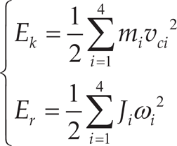
where T is the kinetic energy, which includes the translational kinetic energy E_k and rotational kinetic energy E_r of the four bars as follows:

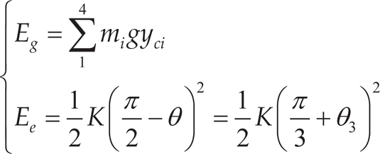
{\begin{cases} E_{k} = \frac{1}{2} \sum_{i = 1}^{4} m_{i} v_{c i}^{2} \\ E_{r} = \frac{1}{2} \sum_{i = 1}^{4} J_{i} ω_{i}^{2} \end{cases}

(6)

V denotes the potential energy including the gravitational potential energy E_g of the bars and the elastic potential energy E_e of the torsion spring. The stiffness coefficient of the torsion spring is K. The free position of the torsion spring is π/2 when there is no energy stored in the spring. The equilibrium position of the spring is 0 rad when it is fully loaded. As illustrated in Figure 2, θ₃ has the following relationship with the angle θ of the torsion spring: θ₃ = θ − 5π/6. θ3 increases from-5π/6 to -π/3 when θ increases from 0 rad to π/2 during the compressing of the spring. E_g and E_e are as follows:

{\begin{cases} E_{g} = \sum_{1}^{4} m_{i} g y_{c i} \\ E_{e} = \frac{1}{2} K {(\frac{π}{2} - θ)}^{2} = \frac{1}{2} K {(\frac{π}{3} + θ_{3})}^{2} \end{cases}

(7)

q_i is the generalized coordinates and Q_i is the generalized forces. When the spring is triggered, the energy stored in the spring is released and the robot obtains an initial velocity for taking off from the ground.

2.2 Simulation

The structural parameters of the body and the main leg cannot be easily modified as they form the robot's main frame, which contains the driving motor, gears, battery, control module, and springs. The lengths of the lower leg and the assistant legs can be modified easily. So, the jumping of the robot is simulated for different values of r₁, r₅, r₁ / (r₁ + r₅), and r₄ with 10 mm length changes to investigate the feasibility of the structural-parameter-based JHD-adjustment method.

In the PRT stage, the generalized coordinates of q_i are [θ₁, θ₂]^T. Two second-order nonlinear differential equations can be derived from (5) as follows:

[\begin{matrix} m_{11} & m_{12} \\ m_{21} & m_{22} \end{matrix}] [\begin{matrix} {\ddot{θ}}_{1} \\ {\ddot{θ}}_{2} \end{matrix}] + [\begin{matrix} c_{1} \\ c {}_{2} \end{matrix}] = [\begin{matrix} Q_{1} \\ Q_{2} \end{matrix}]

(8)

The elements of the matrix and vector in (8) are shown in Appendix A.1. In the POT stage, the generalized coordinates of q_i are [x_f, y_f, θ₁, θ₂]^T. From (5), we can also obtain four second-order nonlinear differential equations, as follows:

[\begin{matrix} m_{11} & m_{12} & m_{13} & m_{14} \\ m_{21} & m_{22} & m_{23} & m_{24} \\ m_{31} & m_{32} & m_{33} & m_{34} \\ m_{41} & m_{42} & m_{43} & m_{44} \end{matrix}] [\begin{matrix} \ddot{x} \\ \ddot{y} \\ {\ddot{θ}}_{1} \\ {\ddot{θ}}_{2} \end{matrix}] + [\begin{matrix} c_{1} \\ c {}_{2} \\ c {}_{3} \\ c {}_{4} \end{matrix}] = [\begin{matrix} Q_{1} \\ Q_{2} \\ Q_{3} \\ Q_{4} \end{matrix}]

(9)

The elements of the matrix and vector in (9) are shown in Appendix A.2.

These equations can be solved by using the ordinary differential equation solver ode45 on MATLAB. The fixed parameters of the robot used in simulations are m₂ = 0.012 kg, m₃ = 0.1 kg, r₂ = 0.079 m, r₃ = 0.033 m, l₂ = 0.0395 m, l₃ = 0.02 m, α = 0.868 rad, J₂ = 2.496e-5 kg m², J₃ = 5.672e-5 kg m², K = 2.1585 N m/rad. The other parameters, r₁, r₄, r₅, l₁, l₄, m₁, m₄, J₁, and J₄, will be decided in the simulations of different adjustment parameters. Linear densities of r₁, r₄, and r₅ are 0.126 kg/m, 0.018 kg/m, and 0.126 kg/m, respectively.

The initial conditions of the PRT stage are θ ₁ = 0 rad, θ₃ = − 2π/3, θ₁ = 0 rad/s, and ${\dot{θ}}_{2}$ = 0 rad/s. θ₂ can be calculated by using r₂, r₃, and θ₃ when r₄ and r₅ are fixed in different simulations. We can get the ending time of this stage when F_y is zero. The initial conditions of the POT stage are x_f = 0 m, y_f = 0 m, ${\dot{x}}_{f}$ = 0 m/s, ${\dot{y}}_{f}$ = 0 m/s, while θ ₁, θ₂, θ₁ and θ₂ are the ending conditions of the PRT stage.

2.2.1 Lower-Leg Length r₁

First, the relationship between the JHD and r₁ is simulated. Here, r₄ = 0.079 m, l₄ = 0.0395 m, r₅ = 0.033 m, and J₄ = 2.975e −6 kg m². l ₁ and J ₁ are decided by r₁, r₅, and m₁ when r₁ changes from 0.065 m to 0.075 m. The jumping trajectories of the robot are shown in Figure 4. The jumping height decreases from 1.59 m to 1.42 m, while jumping distance increases from 0.98 m to 1.91 m when r₁ increases from 0.065 m to 0.075 m. The adjustable ranges of jumping height and distance are 0.17 m and 0.93 m, respectively.

Figure 4.

Jumping trajectories simulation results when r₁ changes

2.2.2 Assistant-Leg-2 Length r₅

The JHD adjustment by r5 is simulated when r1 = 0.07 m, r₄ = 0.079 m, and J₄ = 2.975e-6 kg m2. l₁ and J₁ are decided by r₁, r₅, and m₁ when r₅ changes from 0.033 m to 0.043 m. The simulation results are shown in Figure 5. The jumping height decreases from 1.51 m to 1.26 m while jumping distance increases from 1.47 m to 2.54 m when r₅ increases from 0.033 m to 0.043 m. The adjustable ranges of jumping height and distance are 0.25 m and 1.07 m, respectively.

Figure 5.

Jumping trajectories simulation results when r₅ changes

2.2.3 Ratio r₁/(r₁+r₅)

The JHD also can be adjusted when r1 increases from 0.065 m to 0.075 m while (r₁ + r₅) is 0.103 m and stays constant. Here, r₄ = 0.079 m and J4 = 2.975e-6 kg m2. l₁ and J₁ are decided by r₁, r₅, and m₁. As shown in Figure 6, the jumping height increases from 1.47 m to 1.54 m while jumping distance decreases from 1.85 m to 0.78 m when r₁ increases from 0.065 m to 0.075 m and r₅ decreases from 0.038 m to 0.028 m. The adjustable ranges of jumping height and distance are 0.07 m and 1.07 m, respectively.

Figure 6.

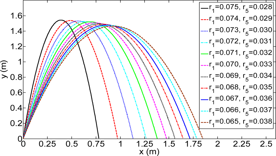
Jumping trajectories simulation results when r1 / (r1 + r5) changes

2.2.4 Assistant-Leg-1 Length r₄

The JHD adjustment by r₄ is simulated when r1 = 0.07 m, r₅ = 0.033 m, and J₁ = 4.597e-6 kg m². l₄ and J₄ are decided by r₄ and m₄. The simulation results are illustrated in Figure 7. The jumping height increases from 1.29 m 1.62 m while jumping distance decreases from 2.28 m to 0.36 m when r₄ increases from 0.073 m to 0.083 m. The adjustable ranges of jumping height and distance are 0.33 m and 1.92 m, respectively.

Figure 7.

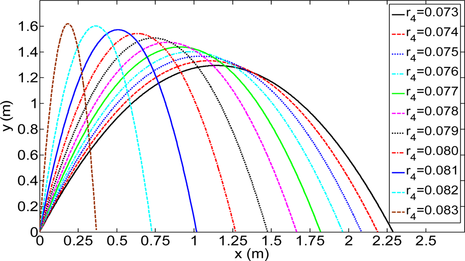
Jumping trajectories simulation results when r₄ changes

Table 1.

Comparison of the four parameters in terms of jumping-height-and-distance adjustable ranges

Adjustment parameter	Variation range(mm)	Height range(m)	Distance range(m)
r ₁	[65, 75]	[1.6, 1.43]	[0.98, 1.9]
r ₅	[33, 43]	[1.5, 1.26]	[1.5, 2.54]
r₁ / (r₁ + r₅)	[65, 75]/103	[1.47, 1.5]	[1.8, 0.78]
r ₄	[73, 83]	[1.3, 1.62]	[2.3, 0.37]

From the simulation results shown in Figures 4 to 7, we can learn that the structural parameters of the four-bar mechanism have significant influences on the robot's jumping performances. A comparison of the adjustments of the four parameters is shown in Table 1. Within the same parameter variation range of 10 mm, r₄ is the most effective adjustment parameter.

3. Jumping-height-and-distance adjustment mechanism design

3.1 Leg-Length Adjustment Mechanisms

Three possible mechanisms for leg-length adjustment are illustrated in Figure 8. L₁, L₂ and L₃ denote the effective length of a leg. In Figure 8 (a),L₁ is adjusted by the angle between L₁₁ and L₁₂ when joint j₁ rotates, driven by a motor. L₂ can be modified by the angle between L₂₁ and L₂₂ when joint j₂ rotates, driven by a motor as shown in Figure 8 (b). In Figure 8 (c),L₃ is changing when the screw L₃₁ is rotating relatively to the nut L₃₂.

Figure 8.

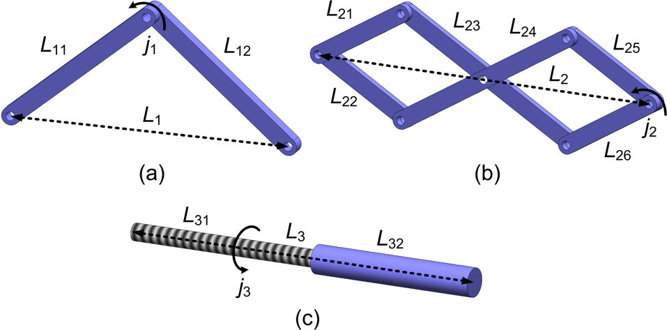
Possible mechanisms for leg-length adjustment. (a) Two-link mechanism. (b) Multi-parallelogram mechanism. (c) Screw-and-nut mechanism.

A comparison of the three mechanisms proposed above is shown in Table 2. The comparison criteria include low number of driving motors, small size, low mechanical complexity, and high mechanical stability. The three mechanisms all need one driving motor. The main advantage of the two-link mechanism is its low mechanical complexity. However, it has the largest size and lowest stability. The multi-parallelogram mechanism has moderate size and stability, but the highest mechanical complexity. The screw-and-nut mechanism has the merits of having the smallest size, moderate mechanical complexity, and highest stability. Thus, the screw-and-nut mechanism is selected as the leg-length adjustment mechanism for our robot.

Table 2.

Comparison of the three leg-length adjustment mechanisms. MC is mechanical complexity. +++ very favourable, ++ favourable, + least favourable.

Method	Size	MC	Stability
Two-link mechanism	+	+++	+
Multi-parallelogram mechanism	++	+	++
Screw-and-nut mechanism	+++	++	+++

3.2 Screw-And-Nut Mechanisms for Leg Adjustment

Screw-and-nut-based mechanisms for the length adjustment of different legs are designed. The CAD models of the mechanisms are shown in Figure 9. In Figure 9 (a), the two lower legs are two screws connected by connectors 1 and 2 with two feet fixed at their end points, respectively. The adjusting motors are mounted on connector 2. Gear 2 is fixed on the screws; gear 1, fixed on the shafts of the motors, is able to drive gear 2. The screws are also driven to rotate relatively to the feet, which have internal thread and can be seen as two nuts. Thus, the length r ₁ of the lower legs can be adjusted when the length r₅ is kept fixed by the bolt.

Figure 9.

CAD models of screw-and-nut mechanisms for the adjustment of the different legs’ lengths. (a), (b), (c), and (d) are mechanisms for adjustment of r₁, r₅,r₁/(r₁+r₅) and r₄, respectively.

In Figure 9 (b), connector 1 can be seen as a nut. The two lower legs are driven by the motors to rotate and r₅ is adjusted when r₁ stays fixed. In Figure 9 (c), the motors are mounted on connector 1. Connector 2 can be seen as a nut which has translational motion along the lower legs while they are rotating. Therefore, r₁ / (r₁ + r₅) can be adjusted. As illustrated in Figure 9 (d), connectors 3 and 4 are connected by a screw. Connector 3 can be seen as a nut which has internal thread. The screw rotates to adjust r₄ when the two connectors do not rotate.

Table 3.

Comparison of the four structural parameters’ adjustment mechanisms. MC is mechanical complexity. EE represents energy efficiency. +++ very favourable, ++ favourable, + least favourable.

Adjustment parameter	Motor	MC	Stability	EE
r ₁	2	+	+	+
r ₅	2	++	++	++
r₁ / (r₁ + r₅)	2	++	++	++
r ₄	1	+++	+++	+++

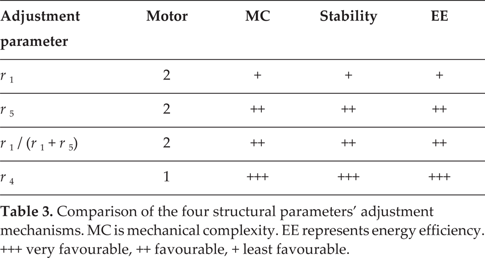
A comparison of the four structural parameters’ adjustment mechanisms is shown in Table 3. The first three mechanisms all need two driving motors and have complex mechanical structures needing synchronized control of the motors. Because the feet will kick the ground before the robot takes off, the connections between the feet and the lower legs are not stable in the r₁ adjustment method. The r₅ and r₁ / (r₁ + r₅) adjustment mechanisms also have the stability problem. The two-mass-model jumping robots have lower energy efficiency when the lower mass accounts for the larger part of the total mass of the robots [23]. The first three mechanisms all need the two driving motors to be mounted near to the lower legs, which represent the lower mass of the model. For thread machining, the lower legs should be made of steel material, which will make the lower mass heavier. Thus, these mechanisms have lower energy efficiency. The last mechanism, adjusting r₄, only needs one driving motor and has the lowest mechanical complexity and the highest stability. The driving motor in the r₄ mechanism is mounted on connector 4, which is close to the body (upper mass) of the robot. The light carbon fibre with high strength used in our previous robot can still be used for the lower legs. Therefore, this mechanism has higher energy efficiency than others. In our robot prototype design and fabrication, we will use this mechanism for JHD adjustment.

3.3 Obstacle Distance and Height Detection

Obstacle-distance-and-height (ODH) information is essential for jumping robots to adjust their JHD. For our 9 cm × 7 cm × 12 cm jumping robot, it is not feasible to install big and heavy distance sensors. The low-weight and small-size SHARP infrared distance sensor GP2D12 with a 10-80 cm detection range is selected and an ODH sensing method is designed. The detection scenario is illustrated in Figure 10. The distance and height of the obstacle are D and H, respectively. The sensor is mounted on assistant leg 1. The yaw and pitch angles are β₁ and β₂. The theoretical distance d is

d = \frac{D}{\cos β_{1} \cos β_{2}}

(10)

The robot steers to find a smallest distance value between itself and the obstacle by adjusting β₁ while keeping β₂ unchanged. Then, the robot adjusts the pitch angle β₂ while keeping β₁ fixed to obtain another smallest distance value, which is the distance D. β₂ has the following relationship with the rotation angle Ψ of the jumping driving motor:

β_{2} = f (ψ)

(11)

For obstacle-height sensing, the detection distance value increases when the torsion springs are compressed and β ₂ is increasing. The critical values β_c and d_c of β₂ and d can be obtained when the output voltage of the sensor is smaller than a pre-set threshold. The height of the obstacle is as follows:

H = d_{c} \sin β_{c} = \sqrt{d_{c}^{2} - D^{2}}

(12)

This ODH detection method will be tested in Section 4.2.

Figure 10.

ODH detection scenario using an infrared distance sensor

3.4 Jumping-Height-and-Distance Adjustment Decision-Making

After establishing the ODH information, the robot has to decide how to adjust its JHD parameters to overcome the obstacle. Assume that the parameters are j_h and j_d, as shown in Figure 11. We need to find the minimum values of j_d and j_h for obstacle overcoming. The trajectory of the robot in the air is a ballistic path. The equation of the trajectory is as follows:

y = - \frac{4 j_{h}}{j_{d}^{2}} {(x - \frac{j_{d}}{2})}^{2} + j_{h}

(13)

In the decision-making process the robot tries to find the required jumping distance J_d and height J_h from the largest value to the smallest value of j_d. Inserting j_d, j_h, and x = J_d = D−Δd when D < j_d / 2 or x = J_d = D + Δ d when D > j_d / 2 (width W of the obstacle is not considered) into (13), we can obtain J_h = y, which should be larger than H + Δ h to make sure the robot can jump over the obstacle. Here, Δd and Δh are respectively set as the width and height of the robot for jumping over the obstacle safely.

Figure 11.

Jumping-distance-and-height adjustment for obstacle overcoming

4. Prototype implementation and experimental results

The prototype of our jumping robot with the new JHD active adjustment mechanism is shown in Figure 12. The new assistant leg 1 is a length-adjustable mechanism, approximately 20 g in weight. The adjusting motor is installed in connector 1, which connects with the body. Connector 2 has a 20-mm-deep internal thread with an infrared distance sensor mounted on its surface. The two connectors are joined together by the screw. First, the adjustment ability of this new mechanism was tested. Then the ODH sensing method was verified by several experiments. Lastly, obstacle-overcoming experiments were done to test the performance of the new version of our robot.

Figure 12.

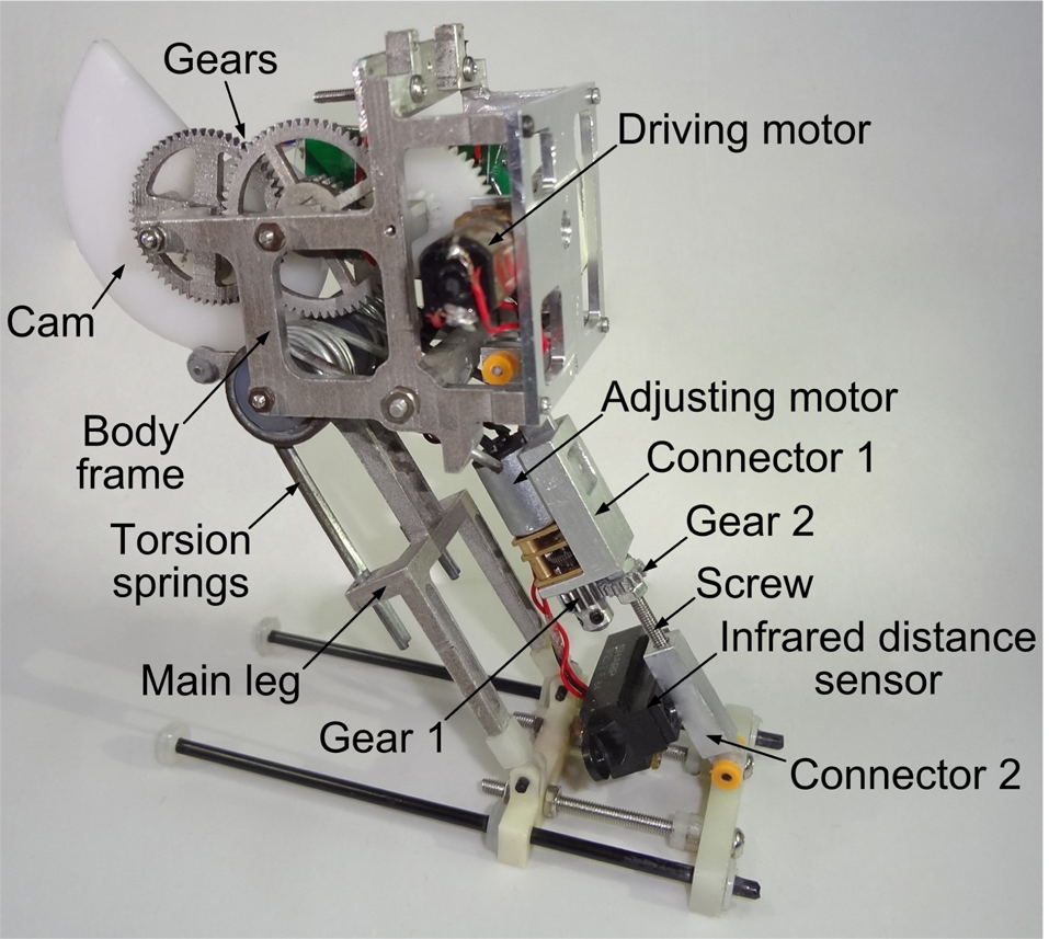
Prototype of our jumping robot with a new JHD active adjusting mechanism

4.1 Jumping-Height-and-Distance Adjustment

Based on the simulation results and the design of the JHD adjustment mechanisms, we first tested the jumping performance with different lengths of r₄ when r₁ = 0.07 m and r₅ = 0.033 m. A board with 80 cm × 125 cm grid coordinates behind the robot was used to estimate the position of the robot in the air. The videos of the jumps with different r₄ were recorded by a Casio high-speed camera with a frame rate of 210 frames/s. The videos were processed by Corel VideoStudio Pro × 4 and the positions of the robot in the air were estimated by comparing the robot's positions with the coordinates on the board. The trajectories of the robot with different lengths of r₄ are shown in Figure 13. The JHD shows the same changing trends as the simulation results, as illustrated in Figure 7. The maximum jumping distance is 0.76 m with the jumping height of 0.87 m when r₄ = 0.073 m. The maximum jumping height is 0.98 m with the distance of −0.2 m when r₄ = 0.083 m. The test results verify the effectiveness of the JHD adjustment method. The differences between the simulation and experimental results will be discussed in Section 5.

Figure 13.

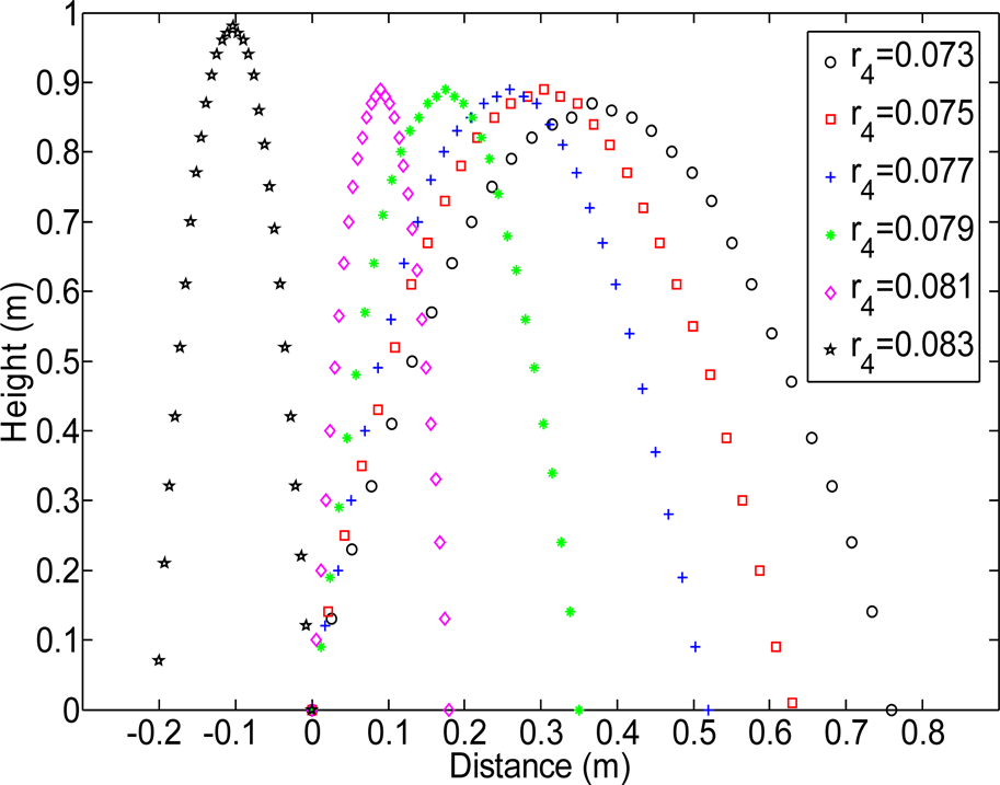
Jumping trajectories of the robot when assistant leg 1 is adjusted by the me echanism with different lengths o f r₄

4.2 Obstacle-Distance-and-Height Detection

Before the obstacle-overcoming tests, the ODH detection method was simulated and tested. The relationship between output voltage v and distance D was tested when the reflected signal of the infrared sensor was perpendicular to the surface of an obstacle. The results are shown in Figure 14. The polynomial-fitting formula of D is as follows:

D = - 2.71 v^{5} + 2.047 v^{4} - 6.046 v^{3} + 8.86 v^{2} - 6.72 v + 2.42

(14)

Then, the sensor was mounted on a two-degree-of-freedom platform to test the distance detection performance of the proposed method when both the yaw angle β₁ and the pitch angle β₂ were changed from −30° to 30°. The simulation and experimental results are shown in Figures 15 and 16 when D is 15 cm and 30 cm, respectively. In the two Figures, (a) shows the theoretical values calculated by using (10), (b) shows the experimental values of distance calculated from the output voltage by using (14), and (c) shows the experimental errors, which are the differences between the experimental values and the theoretical values. The theoretical and experimental values have the same changing trends, as shown in (a) and (b). As can be seen from (c), the maximum errors are 0.0312 m and 0.0448 m at −30° of the yaw angle when D is 15 cm and 30 cm. The largest errors when β₁ = 0° are −0.0181 m and 0.0343 m, which are smaller than the body length of the robot. The robot can make a decision to adjust its jumping distance without considering the detection errors.

Figure 14.

Relationship between the output voltage of the sensor and distance between the sensor and obstacle

From the Figures we also find that the errors are larger when the absolute value of β₁ is larger. This is caused by the non-perpendicular reflecting of the signal of the sensor from the obstacle. Bigger β₁ has more serious influences on the reflected signal. Fortunately, this has only a small effect on D detection because we only need to find the smallest d when the robot tries to steer left and right and pitch up and down.

In order to test the obstacle-height-detection method, one 25-cm-high obstacle and one 45-cm-high obstacle were used. The yaw angle was 0° and the pitch angle increased from −30° to 80°; the output voltages were used to calculate the height h. The results are shown in Figure 17. The test results are close to the calculated results before the critical angles of 55°, 50°, 45°, and 40°, as illustrated in Figure 17 (a). After the pitch angles increase more than the corresponding critical angles for different distances, the test results of obstacle height deviate from the calculated results quickly and the differences between the next values and these values are larger than the 0.05 m threshold. This is because the received signal strength of the sensor drops quickly when β₂ is larger than β_c. So, the tested heights of the obstacle are 0.2202 m, 0.2439 m, 0.2601 m, and 0.2533 m when D is 0.15 m, 0.20 m, 0.25 m, and 0.30 m and β₂ is 55°, 50°, 45°, and 40° respectively. The tested heights are close to the real height of 0.25 m of the obstacle. The maximum error is 0.0298 m when β₂ is 55° and D is 0.15 m. This error has no serious effect on the jumping-height adjustment decision-making of the robot. We can also find that the error is larger when the pitch angle β₂ is larger. Although there are errors, this obstacle-height sensing method is reliable enough and can still be used by the robot to estimate an obstacle's height.

Figure 15.

The theoretical value, experimental value, and the experimental error when D is 15 cm

Figure 16.

The theoretical value, experimental value, and the experimental error when D is 30 cm

Figure 17.

Obstacle height detection results in different distances between the robot and the obstacle

In Figure 17 (b), the results have a similar changing tendency to (a). The tested heights of the obstacl e are 0.3897 m, 0.4002 m, 0.4330 m, a n d 0.4284 m when D is 0.15 m, 0.20 m, 0.25 m, and 0.30 m and β₂ is 70°, 65°, 60°, and 55°, respectively. The tested heights are close to the real height of 0.45 m o f the obstacle. The maximum error is 0.0603 m when β₂ and D are 70° and 0.15 m, respectively. This error also has no serious influence on the robot to adjust its jumping height. The results show that the proposed obstacle-height detection method with one simple distance sensor has higher accuracy when the pitch angle is smaller, which means that the distance D has an influence on the accuracy when the height H is fixed for a given obstacle.

4.3 Obstacle Overcoming

Based on validations of the JHD adjusting and obstacle detection methods, tests for overcoming different heights of obstacle were conducted. Firstly, the relationships among number of rotations n of the adjusting motor, length of r₄, and JHD were investigated. From the test results in Figure 13, we can obtain the relationships between jumping distance j_d and r₄ and jumping height j_h and r₄ as follows:

{\begin{cases} j_{d} = - 6652 r_{4}^{2} + 947 r_{4} - 33 \\ j_{h} = 636570 r_{4}^{3} - 147400 r_{4}^{2} + 11370 r_{4} - 290 \end{cases}

(15)

The pitch p of the screw is 0.5 mm. Gears 1 and 2 all have 16 teeth. r₄ can be expressed by n and p as

r_{4} = r_{40} - n p

(16)

where r₄₀ = 0.083 m is the initial length of r₄. The minimum value of r₄ is 0.073 m. The robot detects the obstacle's height and distance and adjusts the adjusting motor before taking off.

The robot was placed 30 cm in front of obstacles and controlled by the operator wirelessly to detect the ODH when the jumping motor was rotating. The ODH detection results before JHD adjustment are shown in Figure 18. The video sequences of the robot during ODH detection are illustrated in Figure 18 (a). The detected distances are shown in Figure 18 (b). The minimum values of 0.2886 m and 0.3007 m are the detection distances D between the robot and the obstacles when the heights of the obstacles are 28 cm and 48 cm, respectively. Before the sudden increase, the distances of 0.4242 m and 0.5358 m can be seen as d_c. The distance d_c and corresponding D are inserted into (12) to calculate the height of the obstacle. The calculated heights are 0.3109 m and 0.4435 m.

Figure 18.

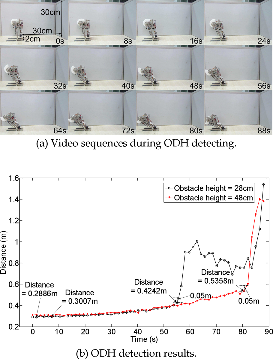
ODH detection before JHD adjusting

j_d and j_h are obtained from (15) for different r₄ when r₄ increases from 0.073 m to 0.083 m. Inserting r₄ = 0.073 m, j_d = 0.7361 m and j_h = 0.8679 m into (13), we can obtain y as 0.6841 m and 0.7093 m when x is 0.2886 m − 0.09 m = 0.1986 m and 0.3007 m − 0.09 m = 0.2107 m respectively (0.09 m is the width of the robot). The values of y 0.6841 m and 0.7093 m are larger than the heights of 28 cm + 12 cm = 40 cm and 48 cm + 12 cm = 60 cm of the obstacles (12 cm is the height of the robot). Hence, the robot can jump over the obstacles with the biggest jumping distance when r₄ is 0.073 m.

The number of rotations n is 20, as calculated from (16). The r₄ length-adjustment video sequences are shown in Figure 19. The motor rotates 20 times in 33 s and r₄ decreases from 0.083 m to 0.073 m. After adjusting the JHD, the jumping motor rotates again and the robot jumps over the obstacles. The trajectory of the robot during flight after taking off for negotiation of the 48 cm height obstacle is shown in Figure 20. The distance between the robot and the obstacle is 30 cm. The JHD are about 87 cm and 76 cm, respectively. The calculated take-off velocity and angle are 4.23 m/s and 77.68°. The obstacle-overcoming test verifies the structural-parameter-based active JHD adjustment method for overcoming different heights of obstacle.

Figure 19.

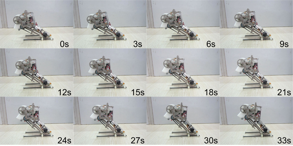
Video sequences of the robot when r₄ decreases from 0.083 m to 0.073 m

Figure 20.

Trajectory of the robot during flight in the air after taking off to overcome a 50-cm-high obstacle

5. Discussion

The jumping heights and distances in the experimental results are smaller than in the simulation results with the same r₄. The energy efficiency is only 58.9% when we compare the initial translational kinematic energies in the test and the simulation results when r₄ = 0.073 m. There are five major causes for the low energy efficiency: the rotational frictions on the joints of the four-bar mechanism, the damping of the torsion springs, the air resistance, the deformations of the cam and lower legs, and the micro-slippage of the robot's feet on the ground before taking off. These five reasons are not considered in the simulation, while they may have serious effects on the jumping performance and the energy efficiency. The first three factors could be considered in the model of the robot. Because the deformation forces of the parts are the functions of the independent variables (angles θ₁ and θ₂), the deformations are not easily integrated into the non-linear differential equations for modelling and simulation. Furthermore, the take-off period is very short; it is therefore difficult to observe the slippage between the feet of the robot and the ground in the experiments. These problems will be studied in our future work.

Another disparity between the experimental and simulation results in jumping is the take-off angle. Comparing Figure 13 with Figure 7, we find that the take-off angles in the tests are larger than in the simulations for the same length r₄. This is mainly caused by the deformation of the lower leg. The deformation of the lower leg can result in the bending backwards of the robot before taking off, and a larger take-off angle.

The proposed structural-parameter-adjustment method for JHD has been verified by simulations and experimental tests. However, this method is still based on the principle of take-off angle adjustment, the same as with the COM adjustment method in our previous robot [14–16]. The jumping height will decrease when the jumping distance increases, which means that the jumping-height adjustment and jumping-distance adjustment are coupled together. This may not be appropriate in some conditions for overcoming higher and more distant obstacles. Two possible solutions could be used to deal with this problem. One would be to design a new uncoupled JHD adjusting method, such as energy controlling for jumping by using the multimodal actuator [24] for jumping robots. The other would be to finely adjust the distance between the robot and the obstacle. This could turn the JHD adjustment problem into a jumping-height adjustment problem only.

The proposed ODH detection method with only one distance sensor is very simple and effective. Its detection accuracy is acceptable for our robot to estimate the ODH before JHD adjustment. The problem is that the obstacle-height detection accuracy decreases when the pitch angle β₂ increases and the signal received by the receiver of the infrared sensor decreases. This means that the robot has higher-precision obstacle-height detection capability when it is located further away from a given obstacle. This problem could be solved if the robot were able to finely adjust the distance between itself and the obstacle.

6. Conclusions and future work

We have presented a jumping-height-and-distance adjustment method based on structural parameter adjusting for a jumping robot overcoming different heights of obstacle. The influences of four possible structural parameters on jumping performances have been simulated. The results show that the length r₄ of the assistant leg 1 has the largest JHD adjustment ranges under the same 10-mm-long changes of the four parameters. Three leg-length adjustment mechanisms have been analysed and the screw-and-nut mechanism selected for the robot. After considering the number of driving motors, mechanical complexity, stability, and energy efficiency, the r₄ adjustment mechanism is selected for our new robot fabrication. The JHD adjustment tests verify the effectiveness of the proposed method. The ODH-detection test results show that this simple method is capable of estimating the distance and height of an obstacle for JHD adjustment decision-making. The results also indicate that the proposed method has higher-precision obstacle-height sensing capability with smaller pitch angle. The obstacle-overcoming test results validate the ODH sensing and the JHD adjustment of our robot.

Future work includes four aspects: (1) Although this prototype of the robot is able to adjust its JHD to overcome different heights of obstacle, the coupling between the JHD adjustments should be solved for flexible obstacle negotiation. A new escape mechanism for jumping should be designed for more fine-grained energy control. Fine motion for position adjustment of the robot as seen with jumping creatures in nature with walking and climbing locomotion modes will also be explored for JHD adjustment decoupling. (2) Reasons for the low energy efficiency will be investigated in depth. The jumping model of the robot will be refined considering the joint frictions, spring damping, air resistance, and deformation of the lower leg. (3) The combinations among the proposed JHD adjustment method of the new robot prototype and the self-righting and steering of the first version of the jumping robot will be studied for cooperative motion planning and continuous jumping locomotion. (4) In order to ensure the robot has a safe landing posture, the active aerial posture adjustment will be studied. Furthermore, the collision energy active absorbing by the leg during landing will be investigated for the next generation of the robot.

7. Acknowledgements

The research reported in this paper was carried out at the Robotic Sensor and Control Lab, School of Instrument Science and Engineering, Southeast University, Nanjing, Jiangsu, China.

This work was supported in part by the Natural Science Foundation of China under Grants 61403079 and 61375076, Natural Science Foundation of Jiangsu Province under Grant BK20140637, International Postdoctoral Exchange Fellowship Program under Grant 20140009, Fundamental Research Funds for the Central Universities under Grant 2242014R20018, and Jiangsu Planned Projects for Postdoctoral Research Funds under Grant 1302064B.

Footnotes

Appendix A

where A, B, A_θ₂, B_θ₂, X₁, X₂, X₃, and X₄ are the same as in Appendix A.1.

References

Armour

Paskins

Bowyer

(2007) Jumping robots: a biomimetic solution to locomotion across rough terrain. Bioinspiration & Biomimetics, 2: 65–82.

Bennet-Clark

(1975) The energetics of the jump of the locust schistocerca gregaria. Journal of Experimental Biology. 63(1): 53–83.

Burrows

(2003) Biomechanics: Froghopper insects leap to new heights - An innovative leaping action propels these bugs to the top of the insect athletic league. Nature. 424(6978): 424–509.

Sutton

and Burrows

(2011) Biomechanics of jumping in the flea. Journal of Experimental Biology. 214(5): 836–847.

Carlési

and Chemori

(2010) Nonlinear model predictive running control of kangaroo robot: a one-leg planar underactuated hopping robot. In: Proc. of IEEE/RSJ Int. Conf. Intell. Robots Syst. Taipei, Taiwan, Oct. 18-22, 2010, pp. 3634–3639.

Nguyen

and Park

(2012) Design and demonstration of a locust-like jumping mechanism for small-scale robots. Journal of Bionic Engineering. 9(3): 271–281.

Liu

Bonsignori

Scarfogliero

(2012) Jumping like an insect: design and dynamic optimization of a jumping mini robot based on biomimetic inspiration. Mechatronics. 22(2): 167–176.

Noh

Kim

(2012) Flea-inspired catapult mechanism for miniature jumping robots. IEEE Transactions on Robotics. 28(5): 1007–1018.

Howe

Obrien

Ambrosi

(2011) The Mars hopper: an impulse driven, long range, long-lived mobile platform utilizing in-situ Martian resources. Acta Astronaut. 69(11-12): 1050–1056.

10.

Dubowsky

Kesner

Plante

(2008) Hopping mobility concept for search and rescue robots. Industrial Robot. 35(3): 238–245.

11.

Ackerman

(2012) Boston dynamics sand flea robot demonstrates astonishing jumping skills. IEEE Spectrum Robot. Blog. http://spectrum.ieee.org/automaton/robotics/military-robots/boston-dynamics-sand-flea-demonstrates-astonishing-jumping-skills.

12.

Cintrón

Pongaliur

Mutka

Xiao

Zhao

, and Xi

(2012) Leveraging height in a jumping sensor network to extend network coverage. IEEE Transactions on Wireless Communications. 11(5): 1840–1849.

13.

Burdick

and Fiorini

(2003) Minimalist jumping robot for celestial exploration. International Journal of Robotics Research. 22(7): 653–674.

14.

Zhang

Song

Qiao

Sun

, and Song

(2012) Self-righting, steering and takeoff angle adjusting for a jumping robot. In: Proc. of IEEE/RSJ Int. Conf. Intell. Robots Syst. 2012 Oct. 7–12; Vilamoura, Algarve, Portugal. pp. 2089–2094.

15.

Zhang

Qiao

Song

, and Wang

(2012) Design and Implementation of a Remote Control System for a Bio-inspired Jumping Robot. International Journal of Advanced Robotic Systems. 9: 1–8.

16.

Zhang

Song

Qiao

Song

, and Wang

(2013) A bio-inspired jumping robot: modeling, simulation, design, and experimental results. Mechatronics. 23(8): 1123–1140.

17.

Steudel-Numbers

and Tilkens

(2004) The effect of lower limb length on the energetic cost of locomotion: implications for fossil hominins. Journal of Human Evolution. 47(1-2): 95–109.

18.

Steudel-Numbers

Weaver

, and Wall-Scheffler

(2007) The evolution of human running: Effects of changes in lower-limb length on locomotor economy. Journal of Human Evolution. 53(2): 191–196.

19.

Pontzer

(2007) Effective limb length and the scaling of locomotor cost in terrestrial animals. Journal of Experimental Biology. 210(10): 1752–1761.

20.

Lim

Babic

and Park

(2008) Optimal jumps for biarticular legged robots. In: Proc. IEEE Int. Conf. Robot. Autom. 2008 May 19–23. Pasadena, CA, USA. pp. 226–231.

21.

Kovac

Fuchs

Guignard

(2008) A miniature 7g jumping robot. In: Proc. IEEE Int. Conf. Robot. Autom. 2008 May 19–23, Pasadena, CA, USA. pp. 373–378.

22.

Zhao

Gao

(2013) MSU jumper: a single-motor-actuated miniature steerable jumping robot. IEEE Transactions on Robotics. 29(3): 602–614.

23.

Zhao

Yang

(2009) Development of a miniature self-stabilization jumping robot. In: Proc. of IEEE/RSJ Int. Conf. Intell. Robots Syst. 2009 Oct. 11–15; St. Louis, USA. pp. 2217–2222.

24.

Leach

Günther

Maheshwari

Iida

, (2014) Linear Multimodal Actuation Through Discrete Coupling. IEEE/ASME Transactions on Mechatronics. 19(3): 827–839.

Structural-Parameter-Based Jumping-Height-and-Distance Adjustment and Obstacle Sensing of a Bio-Inspired Jumping Robot

Abstract

Keywords

1. Introduction

2.1 Modelling

2.1.1 Kinematic Model

3.1 Leg-Length Adjustment Mechanisms

6. Conclusions and future work

7. Acknowledgements

Footnotes

Appendix A

References