State Estimation for Robots with Complementary Redundant Sensors

Abstract

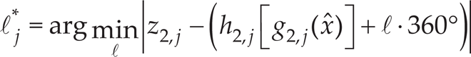
In this paper, robots equipped with two complementary typologies of redundant sensors are considered: one typology provides sharp measures of some geometrical entity related to the robot pose (e.g., distance or angle) but is not univocally associated with this quantity; the other typology is univocal but is characterized by a low level of precision. A technique is proposed to properly combine these two kinds of measurement both in a stochastic and in a deterministic context. This framework may occur in robotics, for example, when the distance from a known landmark is detected by two different sensors, one based on the signal strength or time of flight of the signal, while the other one measures the phase-shift of the signal, which has a sharp but periodical dependence on the robot-landmark distance. In the stochastic case, an effective solution is a two-stage extended Kalman filter (EKF) which exploits the precise periodic signal only when the estimate of the robot position is sufficiently precise. In the deterministic setting, an approach based on a switching hybrid observer is proposed, and results are analyzed via simulation examples.

1. Introduction

Recent technology advances allow to create robots equipped with several kinds of sensors, often providing measures related to the same physical quantity but characterized by quite different and complementary characteristics. The problem of fusing this rich and heterogeneous amount of information can be sometimes far from trivial, and specific techniques, in some cases inspired by biological systems, can be adopted to obtain an effective solution.

An illustrative example in this direction which can be used to introduce the subject is a RFID (radio-frequency identification-based robot localization problem where a reader, installed on the robot, can measure some quantities depending on the distance from a set of RFID tags located in the environment, which act as known landmarks. The use of the RFID technology for robot localization is a recent and promising line of research. RFID data used for localization vary from a binary information (i.e., the tag detection), e.g., [1, 2, 3, 4, 5], to a more complete set of information, like received signal strength indication (RSSI), e.g., [6, 7, 8], or phase shift of the signal, e.g., [9, 10]. The RSSI, often available through quantized levels (e.g., of 1 dBm), usually presents a low sensitivity on the robot-tag distance, with a variation of a few dBm typically only for displacements of the robot in the order of 1 m. The phase shift, on the contrary, is very sharp (typically one degree corresponds to displacements of the robot in the order of 1 mm) but presents a cycle ambiguity, since an unknown number of full wavelengths is contained in the tag-reader distance. Both the measures are then related to the tag-reader distance but present different and, to some extent, complementary characteristics, which should be properly combined to obtain an effective estimation of the robot state.

Redundant and complementary measurements also characterize the perception system of humans and animals, mainly ensuring robustness and reliability. However, more interesting and rich consequences often characterize redundant senses as, e.g., in humans and animals, the presence of two eyes does not simply imply robustness against accidents but also allows to obtain a stereoscopic vision. However, handling this rich set of redundant information can be not trivial from a data processing point of view. More importantly, the information of some senses may be misleading in some situations, and, for this reason, the brain of humans and animals usually faces the problem by inhibiting or activating senses according to the expected importance of the information they can deliver [11]. Well known in this regard is the human pathology known as lazy eye where the brain almost ignores the information coming from a less efficient eye.

Inspired by this biological solution of the problem, we have decided to use this kind of approach to combine redundant sensors with complementary characteristics. In particular, dealing with the RFID-based robot localization problem previously discussed, the direct fusion of the information coming from RSSI and from the phase shift in an extended Kaiman filter does usually provide scarce estimation results. The solution approach proposed here is based on the following scheme: in a first stage, only the imprecise but univocal measurement (e.g., the RSSI in our illustrative example) is used in an extended Kaiman filter to estimate the state of the robot. Only when the estimate starts to become reliable (in a sense that will be specified in the paper), also the other non-univocal measurement (i.e., the phase shift in the considered example) will be incorporated in the Kaiman filter together with the other measure. A dynamic criterion to evaluate the time to switch between the two stages is part of the filtering approach. Notice in fact that also the possibility of resuming the first stage is contemplated by the algorithm. In the deterministic case, a similar approach is proposed by developing a switched observer that exploits both the measures.

Alternative approaches to face the estimation problem addressed in this paper can be developed, resorting to general purpose filtering techniques, e.g., particle filters [12] or multi-hypothesis Gaussian filters (e.g., [13]). These methods may in fact handle the multivariate nature of the measurements considered in this paper. However, these general purpose approaches do not exploit the specific structure of the considered sensory system, whose optimal handling represents a problem dual in a sense to the dynamic allocation of redundant actuators [14]. As a consequence, these approaches usually suffer from a computational complexity point of view, in particular when the size of the state of the system to be estimated becomes large (this occurs, e.g., in a robot localization context where also the coordinates of the landmarks in the environment would be part of the estimation problem).

The paper is organized as follows: in Section II, the problem formulation is provided in the stochastic and deterministic frameworks; the proposed solutions are described in Section III for the two frameworks and numerical simulations are shown and discussed in Section IV.

2. Problem formulation

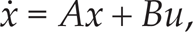
We consider dynamic systems described by the following set of equations:

$\dot{x}=f\left(x,u,w\right),$

(1)

$z_{ij}=h_{ij}\left[g_{ij}(x)\right]+d_{ij},j=1,\dots ,q_i,i=\mathrm{1,2}$

(2)

where x ∊ ℝ ⁿ is the robot state, u ∊ ℝ ^p is a control (or in general a known) input, w ∊ ℝ ^{p _w} is an unknown disturbance acting on the dynamics of the system, z _ij are scalar measures depending on the state, g_ij(x) are scalar functions of the state x (e.g., g_ij(x)= ∥ x ∥), h_ij(⋅) are invertible for i = 1 and periodical with some period Y_j for i = 2 (i.e., h_2j (y + kY _j ) = h_2j(y) for all y ∊ ℝ and k ∊ ℤ), and d_ij are unknown disturbances acting on the measures z_ij.

The idea of the model is that the set of measures Z₁: = {z_1j}_{j=1, …, q1} is such that every measure z_1j ∊ Z₁ is a univocal transformation of some scalar function g_1j of the state x but is affected by a relatively strong disturbance d_1j and/or can be characterized by a low sensitivity on the typical robot displacements in the considered environment. On the contrary, the set of measures Z₂: = {z_2j}_{j=1, …, q2} is such that every measure z_2j ∊ Z₂ is more sensitive and/or presents a better signal-to-noise ratio (i.e., the disturbance d_2j is small if not completely negligible compared to the typical excursion of the signal) but is characterized by a non-univocal dependence on the scalar function g_2j of the state of the system.

2.1 Stochastic scenario

The stochastic scenario will be presented by considering a discrete time version of the original problem. This can be obtained by discretizing (e.g., using an Eulero approximation with some sampling time δ _t ) the continuous time model (1)–(2). In the discrete approximation, any discrete time quantity r_k denotes the corresponding sampled quantity r(kδ _t ). The dynamics reported in Eq. (1) will then be written as follows:

$x_{k+1}=x_k+f\left(x_k,u_k,w_k\right){\delta }_t=:f_d\left(x_k,u_k,w_k\right)$

(3)

The unknown disturbances reported in (3) and in (2) (i.e., w_k and d_ij, for j = 1, …, q_i, i = 1,2) will be assumed 0 -mean Gaussian: w_k ∼ N (0, Q_k) with Q_k a covariance matrix and d_ij ∼ N (0, σ _{d ij} ²).

Moreover, the two sets of measurements Z₁ and Z₂ will be considered coupled in the sense that q: = q₁ ≡ q₂ and, for all j = 1, …, q, g_1j(x)=g_2j(x). To fix ideas, if x_p represents the position of the robot (x_p is usually a subset of the robot state x), these functions will be taken as the distance of the robot from a set of landmarks, i.e., g_1j(x) = g_2j(x) = ∥ x_p − x _{L j} ∥, for j = 1, …, q, where x_Lj are the coordinates of landmark j.

While σ _{d 2j} are assumed negligible, σ _{d 1j} are quite large compared to the typical excursion of the signal (low signal-to-noise ratio). At this regard, for a satisfactory behavior of the estimation process, a key element is the relation between the size of σ_d1j with respect to the h_2j(⋅) period Y_j. As shown in simulation, and as intuitively can be expected, the larger is Y_j w.r.t. σ _{d 1j} for all j, the more effective will be the filtering procedure.

2.2 Deterministic scenario

In the deterministic case, all the variables are not described as random process but deterministic ones. Nevertheless, it is possible to consider unknown disturbances acting on the system dynamics such as w and on the available (redundant) measurements, namely, d. Also in the deterministic case, it is assumed that the magnitude of the measurement disturbances d_1j is considerably larger than d_2j. In particular, d_1j(t) can be even discontinuous in time. Then, we are able to model sensors’ dead zones, letting h_1j(⋅) be continuous with respect to their arguments, even linear if needed, and confine the nonlinear behavior to the signals d_1j's. As an example, if the j-th sensor is affected by a discontinuous dead-zone nonlinearity defined as

${\text{dz}}_{\sigma }(s)\triangleq \{\begin{array}{ll}s\hfill & \text{if}\left|s\right|\ge \sigma ,\hfill \\ 0\hfill & \text{otherwise},\hfill \end{array}$

for some positive scalar σ, we could assume that d_1j(t) is such that

$z_{1j}(t)=h_{1j}\left(g_{1j}\left(x(t)\right)\right)+d_{1j}(t)={\text{dz}}_{\sigma }\left(g_{1j}\left(x(t)\right)\right)$

holds true, with a continuous function h_ij(⋅). Dead-zone and saturation nonlinearities are often associated with low-cost sensors that generally have a (time-varying) nonlinear characteristic for large readings, requiring the use of a saturation, or when high-level noise makes readings close to zero too inaccurate to be acceptable and it is preferable to let the measure equal to zero via a dead-zone nonlinearity. An example that falls into this framework, in case of frequency estimation, is proposed in [15, 16]. In here, which is our starting point with respect to work on multiple output allocation for state estimation and which is far from complete, we consider a very simple system, namely, a first-order LTI (linear time invariant) SISO (single-input-single-output, i.e., p = 1 and q₁ = q₂ in our notation) described by

$\dot{x}=Ax+Bu,$

(4)

$z_1(t)=h_{11}\left(g_{11}\left(x(t)\right)\right)+d_1(t)=Cx(t)+d_1(t),$

(5)

$z_2(t)=h_{21}\left(g_{21}\left(x(t)\right)\right)\text{ }+\text{ }{d}_2(t)\text{ }=\mathrm{mod}\left(g_{21}\left(x(t)\right),Y\right)+d_2(t),$

(6)

where A ∊ ℝ^nxn, B ∊ ℝ ⁿ , C ∊ ℝ^1xn, g₂₁(⋅): ℝ ⁿ → ℝ, and the function mod (s, Y) evaluates the modulus after division of s where Y is the periodicity interval. It is assumed that the output disturbances satisfy the following inequalities:

${\Vert d_1(t)\Vert }_{\infty }\le {\overline{d}}_1,{\Vert d_2(t)\Vert }_{\infty }\le {\overline{d}}_2.$

Despite the simplicity of the considered plant, a number of different considerations can be derived.

3. Proposed solutions

3.1 Stochastic scenario

The idea of the approach is that in a first stage, only the imprecise but univocal measurements z_{1, j}, j = 1,2, …, q are used in an extended Kaiman filter (EKF) algorithm to estimate the state of the robot x. Only when the estimate starts to become reliable (in the sense specified below), also the other non-univocal measurements z_{2, j}j = 1, 2, …, q will be incorporated in the extended Kaiman filter together with z_{1, j}. A dynamic criterion to evaluate the time to switch between the two stages is part of the filtering approach. Notice in fact that also the possibility of resuming the first stage is contemplated by the algorithm. In the case of q > 1, a different stage can be defined for each couple of measures (z_1j,z_2j), i.e., for each landmark j = 1,2, …, q, and the dynamic switching rule could be performed independently on each landmark. This will be discussed below by introducing a simultaneous switching version of the algorithm (where the switching to the second stage is performed simultaneously for all j = 1,2, …, q) and a distributed switching version where the switching to the second stage is performed on a landmark-to-landmark basis.

The following algorithm summarizes the filtering approach. The algorithm is based on a q -dimensional vector, s_k, which denotes the current stage of the filter: s _j,k = 1 if at time step k the algorithm is considering only z_1,j (we say that landmark j is in Stage 1), while s_j,k = 2 if at time step k the algorithm is considering both z_{1, j}, and z_{2, j} (we say in this case that landmark j is in Stage 2). In the simultaneous version of the algorithm, the elements of vector s_k are all simultaneously 1 or 2 (a scalar s_k could be actually used in this case), and it is possible to say, without possibility of confusion, that the algorithm is in Stage 1 or 2.

Given the robot state estimate $\widehat{x}$ , the quantities ž_{1, j} and ž_{2, j}. will denote, respectively, for j = 1,2, …, q the expected measurements z_{1, j}, and z_{2, j}. However, while ž_{1, j} = h_{1, j}[g_{1, j}( $\widehat{x}$ )], more attention should be devoted when dealing with the other measurement in view of the periodicity. In particular, assume g_{2, j}(x)= ∥ x ∥ and h_{2, j}(∥ x ∥) ∊ {-180, 180}. Now, assume that z_{2, j} = h_{2, j} (∥ x ∥) = 178 and that ž_{2, j} = h_{2, j} (∥ $\widehat{x}$ ∥) = −179. Now, this −179° should be probably read as 181°, which is very close to the true measure 178°. As a consequence, in the algorithm, the cycle minimizing the difference | z_{2, j} − ž_{2, j} | has been considered, that is, the expected measurements ž_{2, j} are selected according to the following two equations:

${\ell }_j^{*}=\arg \underset{\ell }{{\displaystyle \min }}\left|z_{2,j}-\left(h_{2,j}\left[g_{2,j}(\widehat{x})\right]+\ell \cdot 360°\right)\right|$

(7)

${\widehat{z}}_{2,j}=h_{2,j}\left[g_{2,j}\left(\widehat{x}\right)\right]+{\ell }_j^{*}\cdot 360°.$

(8)

The switching step presented in the algorithm is a crucial ingredient. A detailed explanation of this part will be reported after the algorithm.

Algorithm 1 Dynamic 2 Stage Extended Kaiman Filter (D2SEKF).

Initialization: Let $\widehat{x}$ ₀ and P₀ be, respectively, the initial estimate of the robot state x and its covariance matrix. Set s_j,0 = 1 for all j = 1,2, …, q and k = 0.

At each time step k, do the following:

• Prediction:

  ${\widehat{x}}_{k+1}^{-}=f_d\left({\widehat{x}}_k,u_k,0\right)$

  (9)
  $P_{k+1}^{-}=F_k{P}_k{F}_k^T+W_k{Q}_k{W}_k^T,$

  (10)

  where F_k and W_k are, respectively, the Jacobian of f_d (x,u,w) w.r.t. the state x and to the noise w computed in the current estimate.

• Correction step:

  $K_{G_1}=P_{k+1}^{-}{H}_{1,k+1}^T{\left(H_{1,k+1}{P}_{k+1}^{-}{H}_{1,k+1}^T+R_1\right)}^{-1}$

  (11)
  ${\widehat{x}}_{k+1}={\widehat{x}}_{k+1}^{-}+K_{G_1}\left(z_{1,k+1}-{\widehat{z}}_{1,k+1}\right)$

  (12)
  $P_{k+1}=\left(I-K_{G_1}{H}_{1,k+1}\right)P_{k+1}^{-}$

  (13)

where R₁ is a diagonal q × q covariance matrix with diagonal elements given by ${\sigma }_{d_{1,j}}^2$ (i.e., the variances of the z_{1, j} measurements), z_1,k+1 = h₁[g₁(x_k+1)] + d_1,k+1 is the vector of measures z_1j= h_{1, j}[g_{1, j}(x_k+1)] + d_1j, ž_1k+1 is the vector of the corresponding expected measures ${\widehat{z}}_{1,j}=h_{1,j}[g_{1,j}({\widehat{x}}_{k+1}^{-})]$ , $H_{1,k+1}$ is the Jacobian of h₁ w.r.t. the state computed in the current estimate, and I is the identity matrix.

If s _j,k = 2 for at least one j ∊ {1,2, …, q], let S_k be the set of landmarks in Stage 2 and let ${\overline{q}}_k$ be the number of the elements in S_k:

$K_{G_2}=P_{k+1}{H}_{2,k+1}^T{\left(H_{2,k+1}{P}_{k+1}{H}_{2,k+1}^T+R_2\right)}^{-1}$

(14)

${\widehat{x}}_{k+1}^{+}={\widehat{x}}_{k+1}+K_{G_2}\left(z_{2,k+1}-{\widehat{z}}_{2,k+1}\right)$

(15)

$P_{k+1}^{+}=\left(I-K_{G_2}{H}_{2,k+1}\right)P_{k+1}$

(16)

where z_2k+1 = h₂[g₂(x_k+1)] + d_2k+1 is the vector of measurements z_2j = h_{2, j}[g_{2, j}(x_k+1)] + d_2j for j ∊ S _k , ž_{2, k+1} is the vector of the corresponding expected measures ž_{2, j} (obtained according to Eqs. (7)–(8)), H_2,k+1 is the Jacobian of h₂ w.r.t. the state computed in the current estimate, R₂ ${\overline{q}}_k\times {\overline{q}}_k$ is a diagonal covariance matrix with diagonal elements given by ${\sigma }_{d_{2,j}}^2$ for j ∊ S_k (i.e., the variances of the z_{2, j} measurements related to landmarks in Stage 2), and I is the identity matrix.

Let finally $\widehat{x}$ _k+1 = $\widehat{x}$ _k+1⁺ and P_k+1 = P_k+1⁺.

c. Stage switching. Two possible switching schemes have been considered: simultaneous and distributed switching.

^* Simultaneous switching (D2SEKFs)

If s _j,k = 1 for all j ∊ {1,2, …, q} and

$\sqrt{H_{1,j}{P}_{k+1}{H}_{1,j}^T}<\frac{Y_j}{n_{\mathrm{\Sigma }}}$

(17)

is met for all j ∊ {1,2, …, q} (where n_σ is a positive constant which value will be discussed in Section 4.1), perform the switching, i.e., set s_j,k+1 = 2 for all j ∊ {1,2, …, q}. Define a counter k_w and set it to 0.

If s_j,k = 2 for all j ∊ {1,2, …, q} and

$\left|z_{1,j_a}-{\widehat{z}}_{1,j_a}\right|>3\sqrt{H_{1,j_a}{P}_{k+1}{H}_{1,j_a}^T+{\sigma }_{d_{1,j_a}}^2}$

(18)

is met for some j_a ∊ {1,2, …, q} or

$\left|z_{2,j_b}-{\widehat{z}}_{2,j_b}\right|>3\sqrt{H_{2,j_b}{P}_{k+1}{H}_{2,j_b}^T+{\sigma }_{d_{2,j_b}}^2}$

(19)

is met for some j_b ∊ {1,2, …, q}, then set k _w = k _w + 1; otherwise, set k_w = 0. If k_w ≥ n_p (where n_p is a positive integer, e.g., n_p = 20 has been considered in the simulative results), return to the first stage, i.e., perform the switching s_j,k+1 = 1 for all j ∊ {1,2, …, q}, and reinitialize the covariance matrix P_k+1 (as discussed below, at the end of Section 3.1).

^* Distributed switching (D2SEKFd)

For every index $j\cancel{\in }{S}_k$ (if any) meeting (17), perform the switching, i.e., set s_j,k+1 = 2. If ${\overline{q}}_k$ = 0, define a counter k_w and set it to 0.

If ${\overline{q}}_k$ > 0 and (18) is met for some j _a ∊ {1,2, …, q} or (19) is met for some j_b ∊ S_k, then set k_w = k_w + 1; otherwise, set k_w = 0. If k_w ≥ n_p, perform the switching s _j,k = 1 for all j ∊ S_k and reinitialize the covariance matrix P_k+1.

The idea of the switching step is as follows. First of all, the quantity $\sqrt{H_{1,j}{P}_{k+1}{H}_{1,j}^T}$ represents the robot position uncertainty in the direction of landmark j. If this uncertainty is small enough compared to the period Y _j , the probability of incurring in a cycle ambiguity becomes negligible. The constant n_σ allows to modulate this probability, and the choice of its value will be discussed in Section 4.1. Figures 1 and 2 provide a graphical description of this concept. The two figures refer to the case where a landmark j is located in the origin of the frame. The robot is measuring z_2j = h_2j(∥ x _p ∥) + d_2j, which is a periodic function of its distance from the origin. The blue curves denote the set of points ξ such that h_2k(∥ ξ ∥) is equal to the measurement obtained by the robot (i.e., the blue curves comprise the points where the robot is expected to be if it measures z_2j and there is no noise in the measurements). Note that the robot (denoted by the green square in the figures), due to the noise d_2j, does not exactly lie on a blue curve but is only close to one of these curves. The ellipses are a graphical representation of the uncertainty associated with the position estimates, reported as small red circles at the center of the ellipses. With probability close to 1, the robot is expected to be within the ellipse. Now, if as in Fig. 1 the uncertainty is too large compared to the period of h_2j, several blue curves intersect the ellipse and it is possible, as illustrated in the figure, that the blue curve near the true robot position is not the curve close to its estimate: in this case, it is possible that the estimate is pushed in the wrong direction, as indicated by the black arrow in the figure, and it is not convenient to use the measurement z_2j. On the contrary, when the estimate is more precise as in Fig. 2, the probability of selecting the wrong curve (i.e., the wrong cycle) becomes negligible, and the estimate is driven in the correct direction. Condition (17) allows to discriminate between the two situations: the quantity reported on the left of this equation is a measurement of the extension of the ellipse in a direction orthogonal to the blue curves, while Y _j , denotes the distance between the blue curves. Assuming n_σ = 1, condition (17) will be not met in the situation of Fig. 1, while it will be satisfied in Fig. 2.

Figure 1.

Due to a large uncertainty in the position estimate, a cycle ambiguity afflicts the estimation process (green square, true robot position; red circle, robot position estimate)

As for the switching from Stage 2 to 1, a similar approach has been considered in the two versions, and, in any case, all s _j,k are simultaneously set to 1 (a more complex approach could be considered where also the switching from Stage 2 to 1 is performed independently landmark by landmark). The idea is that if, for a certain number n _p of consecutive steps (starting from the step where at least one landmark is switched to Stage 2), the innovation of one of the active measurements (i.e., all z_{1, j} with j ∊ {1,2, …, q} and all z_{2, j} with j ∊ S _k ) falls outside a confidence interval, it is necessary to restore Stage 1.

Figure 2.

When the position estimate is precise enough with respect to the period of function h_2j, the probability of incurring in a cycle ambiguity becomes negligible (green square, true robot position; red circle, robot position estimate)

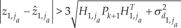
The confidence interval of the innovations is computed as follows. For the measurements z_{1, j} the innovation at time step k can be written as follows:

$\begin{array}{l}{z}_{1,j}-{\widehat{z}}_{1,j}=h_{1,j}\left[g_{1,j}(x_k)\right]+d_{1,j}-\\ -h_{1,j}\left[g_{1,j}({\widehat{x}}_k)\right]\approx H_{1,j}\left(x_k-{\widehat{x}}_k\right)+d_{1,j}\end{array}$

Hence

${\sigma }_{z_{1,j}}^2:=E\left[{\left(z_{1,j}-{\widehat{z}}_{1,j}\right)}^2\right]\approx H_{1,j}{P}_k{H}_{1,j}^T+{\sigma }_{d_{1,j}}^2$

The confidence interval for the innovations on the z_{1, j} measurements is then taken as $[-3{\sigma }_{z_{1,j}},3{\sigma }_{z_{1,j}}]$ . As a consequence, it is the comparison between | z_{1, j} − ž_{1, j} | and 3σ_{z1, j} which dictates the switching from Stage 2 to 1 in the algorithm (a similar expression applies considering the z_{2, j} measurements).

Reinitialization of matrix P _k . After the switching from Stage 2 to 1, the covariance matrix P_k is usually a too optimistic indicator of the real uncertainty associated with the estimate of the robot state. It is for this reason that it is important to reinitialize (increase) its elements. One way could be to reinitialize P_k by taking into account the story of the innovations in the last steps of the filter. A simpler (even if more conservative) way has been adopted in this paper which is based on the fact that, usually, measurements z_{1, j}, due to their univocity, remain reliable during all the execution of the filter. So the uncertainty in the robot state estimate should always remain in the order of the uncertainties associated with these measurements. It is for this reason that in Section 4.1, where a unicycle-like robot is considered, the following choice has been adopted to reinitialize P_k: if x_r = (x, y, θ) denotes the robot state (with x_p = (x, y) being the position of the robot and 0 its orientation), P_k, after the reinitialization, is taken diagonal with elements (1, 1) and (2, 2) (respectively associated with the x − and y -coordinates) given by σ _d ², where σ _d = max _j σ_d1,j. As for the orientation, assuming θ uniformly distributed in (−π, π), a value (2π)²/12 is considered for the element (3, 3) of P _k .

Remark 1 It can be observed how in Stage 2 the two measurementsz_{1, j} and z_{2, j}are not simultaneously incorporated in the EKF but they are processed separately: a first correction of the state is performed using thez_{1, j} measurements, and a successive correction is achieved with thez_{2, j} -based feedback. This choice was motivated by the analysis of some numerical examples, according to which better results were obtained if considering such separate correction.

3.2 Deterministic scenario

Our approach resembles a switched linear observer that can be associated with biological systems that exploit rough measurements to obtain a coarse estimate of the interested quantity (for snakes, it could be represented by odor), and then it is improved by means of more accurate sensors (thermic and tactile perception). Then, we exploit a standard linear observer with output injection formed only by z₁, namely,

$\dot{\widehat{x}}=A\widehat{x}+Bu+K_1\left(z_1-C\widehat{x}\right),\text{if }\left|z_1-C\widehat{x}\right|\ge 2{\overline{d}}_1,$

(20)

with a selection of the gain matrix K₁ ∊ ℝ ⁿ such that A – K₁C is Hurwitz. Note that, defining the estimation error e = x − $\widehat{x}$ , the following inequalities and implications hold true:

$\left|z_1-C\widehat{x}\right|>2{\overline{d}}_1\Rightarrow \left|Ce\right|>{\overline{d}}_1\Rightarrow \text{sign}(Ce)=\text{sign}\left(Ce+d_1\right),$

then sign (z₁ − $\widehat{x}$ ) = sign (Ce). On the same way, it is possible to define a set σ₁(t) ⊂ ℝ ⁿ as

${\mathrm{\Sigma }}_1(t)\triangleq \left\{\widehat{x}\in {ℝ}^n:\left|z_1(t)-C\widehat{x}\right|\ge 2{\overline{d}}_1\right\},$

(21)

so that the observer in (20) is considered when $\widehat{x}(t)\notin {\mathrm{\Sigma }}_1(t)$ . Whenever $\widehat{x}$ is inside the region ${\overline{d}}_1(t)$ , even the sign of the term (z₁ − C $\widehat{x}$ ), which is multiplied by K₁ in (20), is wrong. To move toward the observer dynamics that we propose to use when x ∊ σ₁, we let g₂₁(x) = x₁ and then

$z_2(t)=\text{mod}\left(x_1(t),Y\right)=x_1(t)+{\ell }^{\star }(t)Y,$

for some unknown staircase function ℓ^*(⋅): ℝ_≥0 → ℤ. Then, we propose to use a different output injection whenever $\widehat{x}$ ₁ ∊ σ₁(t) that makes use ¹ of $p:=2{\overline{d}}_1/Y$ admissible values for $\widehat{x}$ according to the measure z₂(t), i.e.,

${\widehat{x}}_{1,\ell }(t)\triangleq {\widehat{x}}_1(t)+\ell Y,$

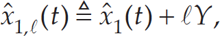
for all integer $\ell \in \mathcal{P}\triangleq [-p,p]$ that by construction is such that ℓ^* ∊ P. To introduce the output injection to be used when x(t) enters ${\overline{d}}_1(t)$ at certain time t₁, we first define the time-varying set

$\mathcal{L}(t)\triangleq \left\{\ell \in \mathbb{Z}:\left|z_1(t)-C{\widehat{x}}_{\ell }(t)\right|\le {\overline{d}}_1\right\},$

(22)

that contains all possible integers ℓ defining the multiple estimates ${\widehat{x}}_{1,\ell }(t)\triangleq {\widehat{x}}_1(t)+\ell Y$ at time t. Note that $\mathcal{L}(t_1)=\mathcal{P}$ . We define a new measure ${\overline{z}}_2(t)$ which is defined as follows:

${\overline{z}}_2=z_2+\zeta Y$

(23)

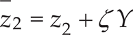
where ζ is such that the new measure ${\overline{z}}_2(t)$ is continuous and has the same time derivatives of z₂(t) almost everywhere. To accomplish this task, ζ is obtained as a hybrid arc solution of the following (switched) hybrid system [17]:

$\dot{\zeta }=0\text{\hspace{1em}if\hspace{1em}}{z}_2(t^{-})=z_2(t^{+}),$

(24)

${\zeta }^{+}=\{\begin{array}{ll}\zeta +1\hfill & \text{if\hspace{1em}}{z}_2(t^{-})>z_2(t^{+})\hfill \\ \zeta -1\hfill & \text{if\hspace{1em}}{z}_2(t^{-})<z_2(t^{+})\hfill \end{array}$

(25)

where z₂(t^±): = lim_{s → t±}z₂(s) and ζ₀ = 0. The resulting ζ is then constant if z₂(t) is continuous in t, whereas ζ is incremented of one if the measure z₂(t) jumps to zero, meaning that its argument is incrementing and then moving to the next periodic interval. On the contrary, it is decremented when z₂(t) has a jump toward its maximum value. To render continuous also the “multiple” estimates x_ℓ(t), it is possible to analogously define

${\overline{\widehat{x}}}_{\ell }={\widehat{x}}_{\ell }+{\zeta }_{\ell }Y,$

where the initial values of ζ_ℓ(0) = ℓ, for ℓ ∊ P, and its flow and jump dynamics are given as in (3.2).

Define a copy ${\mathcal{L}}_0(t)$ of the set $\mathcal{L}(t)$ , ${\mathcal{L}}_0(t_1)=\mathcal{P}$ , where the elements ℓ are successively canceled out if there exists t_2ℓ > t₁ such that $\ell \in {\mathcal{L}}_0(t_{1\ell })$ and $\ell \notin {\mathcal{L}}_0(t_{2\ell })$ . In this way, the cardinality of the set ${\mathcal{L}}_0(t)$ , for all t ≥ t₁, can only shrink and never grow, and the set maintains only the integers that never left the set $\mathcal{L}(t)$ and were contained in $\mathcal{L}(t_1)$ . At time t₁, and since on, we define the observer dynamics to be

$\dot{\widehat{x}}=A\widehat{x}+Bu+K_2\left({\overline{z}}_2-{\left|{\overline{\mathcal{L}}}_0(t)\right|}^{-1}\text{}{\displaystyle \sum _{\ell \in {\overline{\mathcal{L}}}_0(t)}}C{\overline{\widehat{x}}}_{\ell }\right),$

(26)

where ${\overline{\mathcal{L}}}_0(t)$ is the set defined in (22) with ${\overline{\widehat{x}}}_i$ in place of $\widehat{x}$ _i and with cardinality denoted by $|{\overline{\mathcal{L}}}_0(t)|$ . Note that this injection is proportional to the mean value estimation error among the estimates ${\overline{\widehat{x}}}_{\ell }(t)$ for those $i\in {\overline{\mathcal{L}}}_0(t)$ that can be considered admissible with respect to the information given by the measure z₁(t). Note that if the injection term is discontinuous at time instants, the set ${\mathcal{L}}_0(t)$ changes. To conclude, K₂ is designed such that A − K₂C is Hurwitz.

Once the observer dynamics are (26), the output estimation error z₁(t) − C $\widehat{x}$ (t) amplitude is smaller than $2{\overline{d}}_1$ . Note that if ${\overline{d}}_1=0$ and the pair (A, C) is detectable, then the estimation error system e has the origin globally asymptotically stable (GAS) and, when ${\overline{d}}_1>0$ , it is input to state stable (ISS) with respect to the disturbance d₁. These features allow easily to conclude that there exists a time t₁ > 0 such that the set ${\mathrm{\Omega }}_{{\overline{d}}_1}:=\{e\in ℝ:||e+{\overline{d}}_1||\le 2{\overline{d}}_1\}$ is attractive.

Note that we do not attempt here to identify the disturbance signal z₁, given that it could be the signal introduced to model a dead-zone nonlinearity, whose time derivative is represented by means of differential inclusion and not by differential equation, introducing considerable difficulties. This allows also to consider discontinuous signals d₁(t).

For t > t₁, the observer dynamics are (26), and even if (A, C) is observable or detectable, the attractivity of the origin of the estimation error can be lost. Certainly, with the previous assumptions, the estimation error e(t) tends to zero as t goes to infinity if ${\overline{ℐ}}_0(t)=\left\{i^{\star }\right\}$ . As will be shown in the simulation results, the set ${\overline{ℐ}}_0(t)$ shrinks when the noise signal z₁ sufficiently changes in time and spans the amplitudes ranging from $-{\overline{d}}_1$ to ${\overline{d}}_1$ . The control input u, which changes z₁ as well as ${\overline{z}}_2$ , does not help in reducing the set ${\overline{ℐ}}_0(t)$ to identify which one among the estimates ${\overline{\widehat{x}}}_i$ is the right one. Note that even in a very simple case where x is scalar and it is simply described by $\dot{x}=\alpha x+u$ , $y=x+d_1$ , for example, with a constant d₁ ≠ 0, the problem of estimating the state x (and then also d₁) is unsolvable since the problem can be reformulated as the estimation of the state η of a system described by

$\dot{\eta }=\left\{\begin{array}{cc}\alpha & 0\\ 0& 0\end{array}\right\},z_1=[1,1]\eta ,$

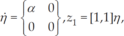
which is unobservable for any α ∊ ℝ when only the measure z₁ is considered.

Remark 2 The proposed approach in both cases (20) and (26) can be indeed rendered a switched high-gain approach selecting change of variables and matrix gainsK₁andK₂as discussed in [18], even for nonlinear systems. Then, the proposed simple approach can be used also in the case of nonlinear systems where semi-global practical results are obtained. Furthermore, since the measurements ofz₂ are essentially not affected by disturbances, the approach proposed in [19] can be pursued in place of (26) to obtain asymptotic results.

These properties noticed by numerical simulations and motivated by intuitive reasoning will be formally addressed in the future.

4. Simulative results

4.1 Stochastic scenario

The robot considered in the simulations is a unicycle-like vehicle with a differential drive kinematics. If x _r,k = (x _k ,y _k ,θ _k ) denotes the robot pose at time step k (with (x _k , y _k ) the position and θ _k the orientation), the discrete time dynamics of the robot can be written as

$x_{r,k+1}=f_d\left[x_{r,k},u_{R,k},u_{L,k}\right]=\left[\begin{array}{l}{x}_k+\frac{u_{R,k}+u_{L,k}}{2}\cos ({\theta }_k)\hfill \\ y_k+\frac{u_{R,k}+u_{L,k}}{2}\sin ({\theta }_k)\hfill \\ {\theta }_k+\frac{u_{R,k}-u_{L,k}}{d}\hfill \end{array}\right]$

(27)

with u _R,k and u _L,k being the distances covered in the time interval (kδ _t , (k + 1)δ _t ) by the right and the left wheels, respectively. The distance u_R,k covered at time step k by the right wheel is related to a noisy encoder reading u _R,k ^e by u _R,k ^e = u_R,k + n_R,k, where the noise term n_R,k is assumed a 0 mean Gaussian random variable with variance given by K_R | u_R,k |, being K_R a positive constant. A similar argument applies to the left wheel. The noise term w_k of equation (3) is then related to the vector of noises (n_R,k,n_L,k). The covariance matrix Q_k associated with (n _R,k , n _L,k ) is a 2 × 2 diagonal matrix with diagonal elements K_R | u_R,k | and K_L | u_L,k |. Similarly, the known input u_k of equation (3) is related to the encoder readings $(u_{R,k}^e,u_{L,k}^e)$ . In this section, K_R = K_L = 2 ⋅ 10⁻² cm and d =26 cm.

The robot moves in a rectangular room with dimensions L₁ × L₂ (with L₁ = 450 cm and L₂ = 350 cm). Assume that there are three landmarks in the environment, with coordinates, respectively, given by [x₁,y₁] = [0,0], [x₂,y₂] = [L₁,0], and [x₃,y₃] = [0,L₂]. The robot measures the distance to each landmark j = 1,2,3:

$\begin{array}{l}{z}_{1j}=h_{1,j}\left[g_{1j}\left(x,y\right)\right]+d_{1j}=g_{1j}\left(x,y\right)+d_{1j}=\\ =\sqrt{{(x-x_j)}^2+{\left(y-y_j\right)}^2}+d_{1j}\end{array}$

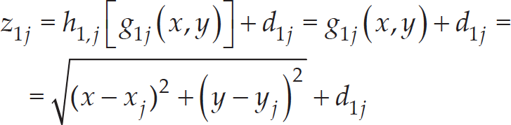
and a periodic function of the distance:

$z_{2j}=mod\left(2\pi g_{1j}(x,y)/Y_j+d_{2j},2\pi \right).$

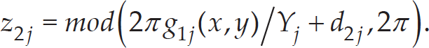
So z_2j ∊ [0,2π]. The quantity Y_j represents the metric period of z_2j, that is, two points with distances from landmark j which differ by a multiple of Y_j will have the same measure z_2j. The value of Y_j will be specified below in the different simulations considered. The noise terms $d_{1j}\sim N(0,{\sigma }_{d_{1j}}^2)$ and $d_{2j}\sim N(0,{\sigma }_{d_{2j}}^2)$ are 0 mean independent Gaussian random variables, with ${\sigma }_{d_{1j}}=50$ cm and ${\sigma }_{d_{2j}}=5°$ for all j = 1, …, q. These numerical values have been inspired by the RFID application in [9].

In Fig. 3, considering only landmark 1 and a measurement z_2,1 = 90.8°, it is reported the set of points characterized by this value of z_2,1 (in absence of noise): that is, in all the circles (dashed and solid) reported in the figure, z_2,1 = 90.8°. The circles have radius a + i ⋅ Y₁, i = 1,2, …, where a = 5.04 cm is the radius of the smallest circle corresponding to a phase of 90.8° and Y₁ = 20 cm. Notice how the periodicity Y₁ is such that, due to the standard deviation of d_1,1 (which is 50 cm), several circles may correspond with high probability to a given couple (z_1,1,z_2,2). For example, if the observed z_1,1 was 285 cm and, due to the noise in z_1,1, all the distances in the interval [z_1,1 − σ_d1,1,z_1,1 + σ_d1,1] = [235,335] cm are considered possible with high probability, the solid circles in the figure represent the robot positions associated with the couple (z_1,1,z_2,2) = (285cm, 90.8°).

Under this setting a first simulation is considered where the robot covers a random path of 1000 steps, assuming Y_j = Y = 20 cm for all j = 1,2,3. The random path of the robot is obtained as follows: the robot moves on straight lines (covering 1 cm in each simulation step) and performs a random curve whenever its distance from the border of the environment becomes less than 1 m. The initial pose of the robot x _r ,₀ = [100cm,70cm,0°] ^T is completely unknown, and the algorithm is initialized, taking as initial estimate $\widehat{x}$ _r,0 = [0,0,0] ^T characterized by a diagonal covariance matrix P₀ with diagonal elements given by L₁²/12, L₂²/12, and (2π)²/12. In Fig. 4, a comparison is reported between the position estimation error

Figure 3.

Landmark 1: in all the circles represented in the figure (dashed and solid), z_2,1 = 90.8°. Here, the periodicity is Y₁ = 20 cm. The solid circles are the more likely circles associated with the couple (z_1,1,z_2,2) = (285 cm, 90.8°)

$e_k=\sqrt{{\left({\widehat{x}}_k-x_k\right)}^2+{\left({\widehat{y}}_k-y_k\right)}^2}$

obtained when using an EKF based only on z_1j(j = 1,2,3) and the error obtained using the simultaneous switching version of Algorithm 1, with n_σ = 4 (the figure also reports the error obtained by integrating the encoder readings starting from the correct initial pose of the robot). It can be observed how the estimation error of the proposed approach gets much smaller at step 229 where the switching from Stage 1 to 2 occurs. Notice that an EKF which uses both z_1j and z_2j (j = 1,2,3) from the beginning would produce a very poor performance (average estimation error in the order of 80 cm) since it would reconstruct a parallel robot trajectory starting from the considered initial position estimate (0,0).

Figure 4.

The position estimation error e _k produced by an EKF exploiting only measurements z_1,j (blue dashed), using the simultaneous switching version of Algorithm 1 (red solid) and the odometry integration from the correct robot pose (black dotted)

In Fig. 5, the same path of Fig. 4 has been considered, but a jump of 20 cm in the y -coordinate of the robot position has been introduced at step 500. The size of the jump and the time when it occurs are completely unknown to the estimation algorithm (kidnapping problem) which is able to automatically detect it through a persistent inconsistency in the innovations. In fact, from Fig. 5, it is possible to see the capability of the algorithm to restore Stage 1 a few steps after the jump.

Figure 5.

Kidnapping problem: a jump has been introduced on the robot path (blue curve) at step 500. The simultaneous switching version of Algorithm 1 is able to detect it and to restore Stage 1. The red plot is the estimated robot position with the algorithm in Stage 1 and the green plot with the algorithm in Stage 2. The red stars are the three landmarks.

Considering a longer random path (5000 steps), the steady-state performance (defined as the mean of the position estimation errors e_k in the last 2500 steps of the simulation) of the simultaneous switching version of Algorithm 1 has been evaluated by performing 100 independent simulation runs for each value of n_σ ∊ {1,2,4,6} and Y ∊ {1,2, …, 50} cm. In Fig. 6, the ratio p between this performance and the one given by an EKF which only uses z_1j for the considered values of n_σ and Y is reported. A ratio equal to 1 means that the proposed approach does not improve the estimate obtained by the EKF which only uses z_1j, and this corresponds to the fact that a switching to the second stage of the filter did not occur. A value less than 1 means that the filter is switched to Stage 2. From the figure, it can be seen how, increasing n_σ, a larger period Y_j is required to allow the switching from Stage 1 to 2 (according to Eq. (17)). However, small values of n_σ may cause a too optimistic switching: the filter enters Stage 2, but the estimate is yet not enough precise to allow the use of the measurements z_2j. This causes the filter to return to Stage 1.

For Y > 20 cm, all the simulations, with any value of n_σ, have switched to Stage 2 and provide a similar performance, with an error which is less than 5% of the error obtained with the EKF based only on the z_1j. Notice however that,

Figure 6.

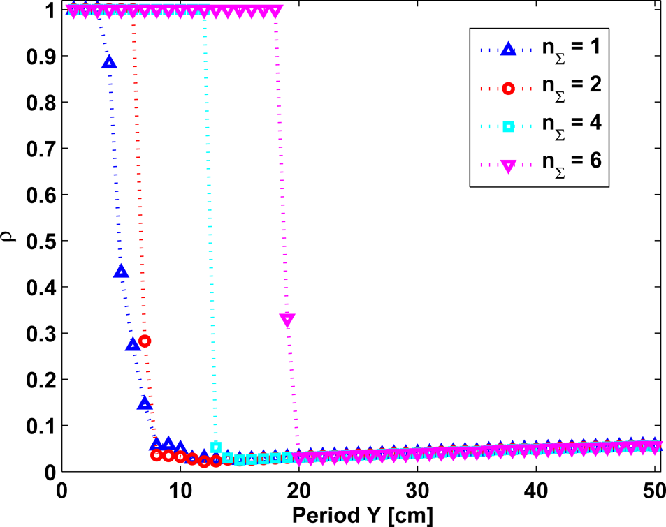
Ratio ρ between the performance of the simultaneous switching version of Algorithm 1 and the one given by an EKF which only uses z_{1 j} for different values of n_σ and Y

for Y < 20 cm, all the curves are slightly increasing: this depends on the fact that the standard deviation on the z_2j measurements has been taken of 5° which corresponds to a larger distance as Y increases. More in detail, if Δ _Y represents the metric standard deviation in the z_{2 j} measurements corresponding to s_{d2 j}, we have Δ _Y = 5Y /360. So, with Y = 20 cm, a standard deviation of 5° corresponds to Δ _Y = 0.28 cm, while for Y = 50 cm, we have Δ _Y = 0.69 cm.

It is also interesting to examine the average of the switching times from Stage 1 to 2 of the proposed approach for different values of n _σ and Y. The average of the switching times has been computed over the same set of simulations considered in Fig. 6 and is reported in Fig. 7. From the figure, as expected, it can be seen how the switching times are decreasing with Y and increasing with n_σ. For small values of Y and/or large values of n_σ, the switching did not occur in all or some of the 100 simulations: in these cases, the average is not defined and is then not reported in Fig. 7.

It has been mentioned how the switching time from Stage 1 to 2 becomes larger when the value of n_σ is increased and how small values of n_σ may cause too premature switchings with the consequence that the algorithm is forced to return to Stage 1. In Table 1, the percentage of the correct switchings from Stage 1 to 2 performed by the proposed approach as a function of n_σ is reported. A switching from Stage 1 to 2 is considered correct if it is not followed in the considered simulation by a switching from 2 to 1. The percentages reported in Table 1 have been computed over the same set of simulations considered in Figs. 6 and 7. Actually, in the simultaneous switching version of the approach, a value of n_σ = 4 allows to obtain a correct switching in the 100% of the cases. The minimum period Y required to obtain a safe switching turns out to be about 13 cm (i.e., Y = 13 cm is the minimum value of Y which, with n_σ = 4, allowed to obtain

Figure 7.

Average switching times from Stage 1 to 2 of the proposed approach (simultaneous switching version) for different values of n_σ and Y

in all the 100 simulations considered a switching to Stage 2, while for all Y < 13 cm, a switching was never obtained in all the 100 simulations). Notice that the minimum Y is very small if compared to the standard deviation σ_d1j which is 50 cm. This depends on the fact that more landmarks are considered and a filtering approach in general allows to significantly reduce the uncertainty associated with each single measurement (more precisely, the steady-state covariance matrix associated with the estimate of the robot position is such that the steady-state variance of the estimates of the distances to the landmarks is less than Y / 4 for Y ≥ 13 cm).

Table 2 reports the percentage of success obtained if considering the distributed switching version of Algorithm 1 (a 0 percentage of correct switching has been observed with n_σ = 1 and 2). It is interesting to see how larger values of n_σ are required when considering the distributed approach if compared to the simultaneous approach. This depends on the fact that when the switching is performed on a landmark by landmark basis, it is sufficient that the variance of the estimate of the distance to just one landmark j becomes smaller than Y_j/n_σ to perform the switching from Stage 1 to 2 of that landmark. Instead, in the simultaneous version of the algorithm, the variance of the estimate of the distances to all the landmarks must become less than Y _j /n_σ simultaneously.

Table 1.

Percentage of correct switchings from Stage 1 to 2 when using the simultaneous switching version of Algorithm 1

nσ = 1	nσ = 2	nσ = 4	nσ = 6
10%	76%	100%	100%

Table 2.

Percentage of correct switchings from Stage 1 to 2 when using the distributed switching version of Algorithm 1

nσ = 4	nσ = 6	nσ = 9	nσ = 12
3%	42%	89%	96%

Figure 8.

The quantity $\sqrt{H_{1,j}{P}_k{H}_{1,j}^T}$ (black solid) and the corresponding thresholds Y_j/4: (blue dash-dot) when using the simultaneous switching version of Algorithm 1: a switching to Stage 2 is not possible since $\sqrt{H_{\mathrm{1,1}}{P}_k{H}_{\mathrm{1,1}}^T}$ is always larger than Y₁/4

Figure 9.

The quantity $\sqrt{H_{1,j}{P}_k{H}_{1,j}^T}$ and the corresponding thresholds Y_j/15 when using the distributed switching version of Algorithm 1: the switching times to Stage 2 for landmarks 1, 2, and 3, respectively, occur at time step 637, 356, and 355

According to the tables, a value of n_σ = 4 has been adopted when using the simultaneous switching version of Algorithm 1, and n_σ = 15 has been adopted in the other case. These values of n_σ allow to obtain, using the corresponding approach, a correct switching from Stage 1 to 2 with a probability close to 1. However, the distributed switching version of the algorithm is usually characterized by a smaller switching time being the switching from Stage 1 to 2 of a landmark triggering in a few steps the switching of all other landmarks. For example, considering again the simulation of Fig. 4, while the switching from Stage 1 to 2 of the simultaneous approach occurred at step 229 (as seen in Fig. 4), using the distributed switching approach, the following switching times for landmarks 1, 2, and 3 were, respectively, observed: 69, 72, and 72.

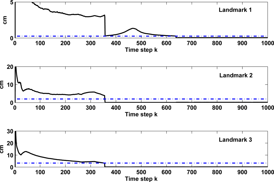
In any case, the real advantage of the distributed switching version of the algorithm, as explained in Section 3.1, can be appreciated when the Y_j are different. For example, in the same setting of Fig. 4, assume now that Y₁ = 4 cm, Y₂ = 30 cm and Y₃ = 50 cm. All other parameters remain as in the simulation of Fig. 4. The very small value of Y₁ implies that the simultaneous version of Algorithm 1 will never be able to switch to Stage 2: in fact, the projection on the distance to the first landmark of the steady-state covariance matrix associated with the robot position estimate based only on the measurements z_1j, j = 1,2,3, never becomes less than Y₁/4 (see Fig. 8). On the contrary, the distributed version of the algorithm allows to obtain rather quickly the switching to Stage 2 of landmarks 2 and 3. Thanks to these additional precise measurements, the covariance gets reduced and, after some steps, also the switching to Stage 2 of the first landmark becomes possible. This is illustrated in Fig. 9, which reports the behavior of the quantity $\sqrt{H_{1,j}{P}_k{H}_{1,j}^T}$ and the corresponding threshold Y_j/15. From the figure, it can be observed how the first switching to Stage 2 concerns the third tag, which is the one associated with the largest period Y₃ = 50 cm, and occurs at time 355. This immediately allows to get the switching of landmark 2 at step 356. Thanks to these new measurements, the covariance matrix is immediately reduced at step 357 and also the quantity $\sqrt{H_{\mathrm{1,1}}{P}_k{H}_{\mathrm{1,1}}^T}$ (i.e., the one associated with landmark 1) gets very close to Y₁/15. However, a value $\sqrt{H_{\mathrm{1,1}}{P}_k{H}_{\mathrm{1,1}}^T}=0.278$ larger than Y₁/15 = 0.267 does not allow the switching also of the first landmark which actually occurs later, at step 637. While a steady-state error of 5.21 cm was obtained with an EKF only based on the rough measurements z_1,j (and also by the simultaneous switching version of Algorithm 1 which is not able in this case to perform the switching to Stage 2 as illustrated in Fig. 8), an estimation error of only 0.25 cm is obtained by the distributed switching version of Algorithm 1. Notice that the use of the measurement z_2,1, i.e., the very precise periodic measurement associated with the first tag, allows to significantly reduce the estimation error: if this measurement was ignored, the distributed switching version of Algorithm 1 would obtain a steady-state estimation error of 0.56 cm.

4.2 Deterministic scenario

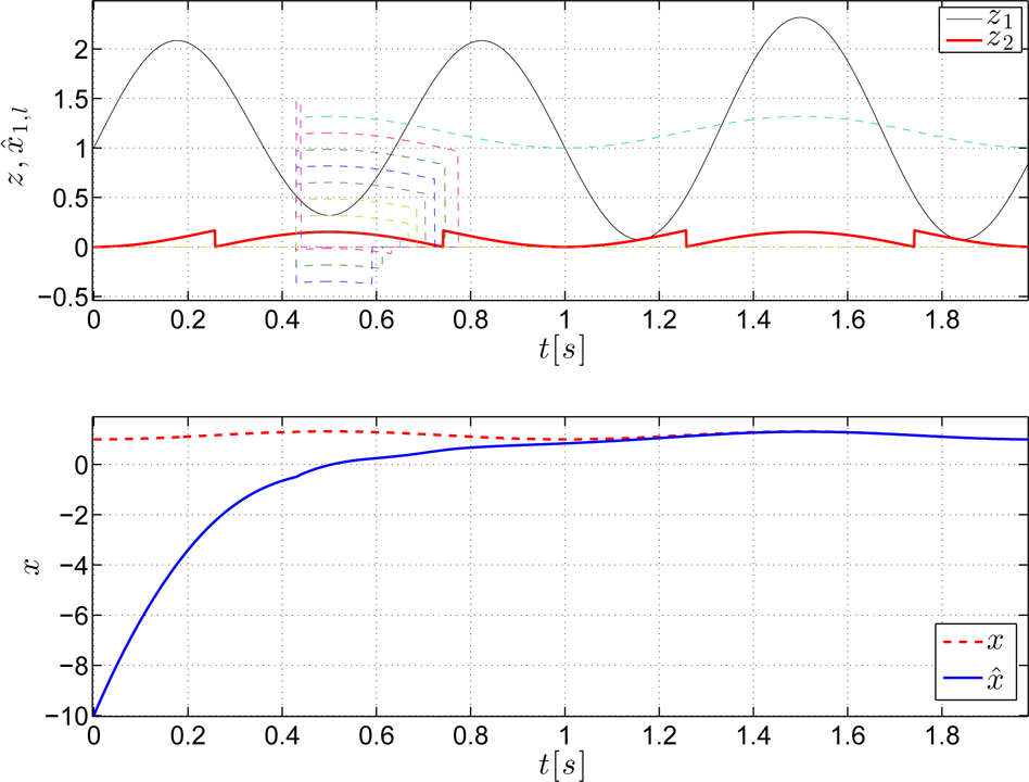
To provide a simple and intuitive example to appreciate the interesting properties of the proposed solutions, we have considered a simple first-order system with A = 0, B = 1, and C = 1, the control u = sin(2πt), the disturbance acting on the measure z₁ such as $d_1=0.5\sin (2\pi 1.5t)$ and $Y={\overline{d}}_1/3$ . The observer matrix gains are selected as K₁ = 4 and K₂ = 10. In the simulation results shown in Fig. 10, the estimated value of $\widehat{x}$ (t) asymptotically (exponentially) converges toward x(t) although the set ${ℐ}_0(t)$ does not converge on a single element, i.e., there are multiple possible selections ${\overline{\widehat{x}}}_i$ that do not disagree (through the inequality (22)) with the measure z₁. This is caused by the fact that ${\overline{d}}_1=1$ (double) larger than the actual maximal amplitude of the disturbance d₁ is considered. Nevertheless, since the disturbance d₁ has zero mean value and this is captured by the input injection in (26), the estimation error converges toward zero.

The second simulation shows in Fig. 11 that if a tight bound on the z₁ amplitude is known, i.e., ${\overline{d}}_1=\left|\right|z_1(t{)||}_{\infty }$ , when the disturbance amplitude spans between $-{\overline{d}}_1$ and ${\overline{d}}_1$ , the set of the admissible estimates ${\overline{\widehat{x}}}_i$ shrinks toward a single element. The last numerical simulations in Fig. 12 show that whenever the disturbance d₁(t) has no zero mean value, even if the tight bound ${\overline{d}}_1=\left|\right|d_1(t{)||}_{\infty }$ is known, a constant estimation error is induced. This is given by the intrinsically symmetric (zero mean) condition in the definition of the set $ℐ(t)$ and the fact the d₁(t) = 0.7sin(2π1.5t) + 0.3 has a constant (unknown) term.

Figure 10.

Top plot: the measures z₁(t) and z₂(t) are shown in black and red solid lines, respectively. Approximately at time t₁ = 0.5 s, the observer dynamics is switched from (20) to (26) and some of the estimates ${\overline{\widehat{x}}}_i$ , corresponding to the measures ${\overline{\widehat{z}}}_{2,i}={\overline{\widehat{x}}}_i$ , depicted in dashed colored lines, do not satisfy the constraint in $\overline{ℐ}(t)$ and are canceled out. Bottom plot: the estimated value $\widehat{x}$ (t) converges to x(t) although $\left|{\overline{ℐ}}_0\left(t\right)\right|$ does not converge to one since the disturbance d₁(t) has zero mean value.

5. Conclusions

In this paper, the problem of fusing the information coming from two typologies of redundant sensors with complementary characteristics has been considered. The two types of sensors provide a measure related to the same quantity but possess different and, to some extent, complementary characteristics: the first one is rough and may be large grain and/or present a low sensitivity on the dynamics of the robot. The second type of sensor, on the contrary, even if precise, is supposed to present a non-univocal dependence on the robot state. This kind of situation also characterizes humans and animals where some perception organs are duplicated. In some cases, the biological solution adopted to face the problem of fusing the information is to inhibit or activate senses based on the expected importance of the information they deliver at the moment. Inspired by this approach, in the stochastic context, a two-stage extended Kaiman filtering algorithm is proposed which, in a first stage, only uses the imprecise but univocal measurement and, only when the estimate starts to become reliable, also incorporates the other non-univocal measurement in the filter. The direct fusion of the two measures in a standard Kaiman filter would often provide scarce results. In the deterministic setting, a similar approach has been shown to yield effective results and stimulating new possible strategies and interesting properties of the considered problem. Future developments could include an analytical investigation of the observability and the detectability properties of the considered problem.

Figure 11.

Contrary to Fig. 10, ${\overline{d}}_1$ has been picked equal to the maximal amplitude of the disturbance d₁(t), i.e., ${\overline{d}}_1=\left|\right|d_1(t{)||}_{\infty }$ . In this case, since the d₁(t) reaches values from $-{\overline{d}}_1$ up to $-{\overline{d}}_1$ , only one admissible estimate ${\overline{\widehat{x}}}_i$ is maintained, and at time 0.8s, the set ${\overline{ℐ}}_0(t)$ has only one element.

Figure 12.

In this case, we considered a disturbance with no zero mean value, namely, d₁(t) = 0.7sin(2π1.5t) + 0.3 and ${\overline{d}}_1=1$ , yielding a constant error