Magnetic localization during manipulation by two robotized permanent magnets

Abstract

Localization methods for magnetically actuated medical robots have long been a topic of research, as they are fundamental to closed-loop control and delivery of functionalities. However, magnetic localization has mainly been linked to robots under a single permanent magnet control. With the release of multi-magnet actuation systems for increased control and manipulability, new localization methods are needed to account for the added magnetic field sources. This paper presents a six degree of freedom localization method for magnetically actuated robots under two external permanent magnets control. The approach relies on the measurements of an accelerometer and gyroscope for the estimation of orientation in the Special Orthogonal Group SO (3), and the measurements of the actuating magnetic fields for the estimation of position. The observability analysis of the system is presented, and the relationship between the external permanent poses and conditioning of the system is explored. Additionally, a calibration procedure to determine the relative poses between the two external permanent magnets is presented where the path that the magnets travel is optimized for the best results. Lastly, the localization method was implemented in a magnetic soft continuum robot and achieved positional average errors of 3.5 mm in norm, and orientation errors of 2.5°, 1.5°, and 2.8° around x, y, and z, respectively.

1. Introduction

Medical and surgical robots have seen significant development over recent decades as they are able to reduce procedural times and learning curves for clinicians, while increasing patient comfort through less bleeding and scarring. The use of magnetic fields for actuation has sparked increased interest as it allows for remote actuation and miniaturization without loss of controllable degrees of freedom (DOF) (Hu et al., 2018; Nelson et al., 2022; Salmanipour et al., 2020; Xu et al., 2019). The development of soft magnetic continuum robots (SCR) capable of reaching deeper inside the human body in a safe and autonomous manner has further advanced the state of minimally invasive robotic surgery (Kim et al., 2022; Koszowska et al., 2023; Wang et al., 2022).

Given the high non-linearity of magnetic fields, localization of magnetically actuated medical robots (MAMR) is fundamental to ensure accurate actuation and manipulation. Additionally, it enables closed-loop control (Mahoney and Abbott, 2016; Pittiglio et al., 2023b; Xu et al., 2022b), autonomous navigation (Martin et al., 2020), and delivery of functionality (Norton et al., 2019). However, the majority of commercially available localization systems are either not compatible with magnetic actuation (e.g., electro-magnetic tracking) or rely on imaging methods, such as fluoroscopy (Bianchi et al., 2019; Wu et al., 2023) or ultrasound (Pane et al., 2022). As such, the topic of localization of magnetic robots has been heavily researched and developed (Dupont et al., 2021; da Veiga et al., 2020), with significant work on achieving both actuation and localization using the same magnetic fields (Fischer et al., 2022a; Popek et al., 2016; Son et al., 2019; Taddese et al., 2018).

For this, the use of magnetic field sensors has been crucial. From multi-sensor arrays to a single sensor placed internally to the MAMR, these solutions have been able to provide localization in a relatively low-cost and easy to implement manner. In conjunction with magnetic field sensors, the use of an inertial measurement unit (IMU) containing an accelerometer and gyroscope has been shown effective in the 6-DOF pose estimation of endoscopic capsules (Di Natali et al., 2016). However, these have generally been confined to actuation systems either consisting of a single external permanent magnet (EPM) or electromagnetic coils (Bianchi et al., 2019; Boehler et al., 2022; Son et al., 2019; von Arx et al., 2023). The drive for enhanced actuation has led to the advent of actuation platforms based on multiple EPMs, such as the FDA approved Steoreotaxis Genesis RMN® (Carpi and Pappone, 2009), the dual External Permanent Magnet (dEPM) platform (Pittiglio et al., 2022a), or multiple rotating PMs (Ryan and Diller, 2017). Due to the increased complexity of the resulting magnetic field, fluoroscopy is still the standard localization practice as newer magnetic field based methods for such platforms have been lacking (Nelson et al., 2022). Only recently a 3D position magnetic localization system was demonstrated under optimized magnetic field gradients (Fischer et al., 2022a), with an additional feasibility study on using an array of magnetic field sensors for the full 6-DOF localization (Fischer et al., 2022b). Additionally, the feasibility of magnetic localization with respect to multiple EPMs was investigated (da Veiga et al., 2023). This work, however, failed to provide a solution compatible with simultaneous actuation and localization, being limited to quasi-static or slow moving MAMR only (refresh rate of 2.5 Hz). Real-time localization is essential in a surgical context where constant tool localization is required for patient safety. Additionally, the implementation of increasing levels of computer assistance toward autonomy generally requires closed-loop control which, in turn, needs localization refresh rates above 100 Hz to run smoothly (Mahoney and Abbott, 2016; Taddese et al., 2018). The use of superimposing oscillating magnetic fields for localization and actuation has shown promising results in electromagnetic coil systems, although at a slower refresh rate of 10 Hz (von Arx et al., 2023).

This work, to the best of the authors’ knowledge, introduces and implements for the first time a real-time 6-DOF pose estimation algorithm for MAMR under dEPM control based on the actuation magnetic fields. This was achieved by, first, carrying out an observability analysis of the problem, followed by defining the singularity regions across the workspace when two EPMs are present. Unlike single-EPM systems for which the constant singularity regions have been well defined and solved for (Taddese et al., 2018), multi-EPM systems suffer from variable singularity regions depending on the current relative pose of the EPMs under which localization becomes challenging. We show how these singularity regions can be avoided while maintaining full control of the MAMR. Finally, the localization algorithm was tested on an SCR under actuation in the dEPM platform. Generally, SCR have their navigation constrained by the surrounding environment limiting their range of motion and speed (Koszowska et al., 2023; Pittiglio et al., 2023a). Therefore, we have tested our localization algorithm in open-space in order to fully showcase the algorithm’s ability to cope with quick and large state changes.

2. Observability analysis

We consider finding the pose of a MAMR, with frame { $\mathcal{A}$ } within the workspace of a dEPM platform with reference frame { $\mathcal{W}$ } (see Figure 1). We consider the EPMs to be cylindrical and axially magnetized, and that the MAMR is fitted with a 3D accelerometer, 3D gyroscope, and a 3D Hall effect (HE) magnetic field sensor.

Figure 1.

Representation of the world reference frame {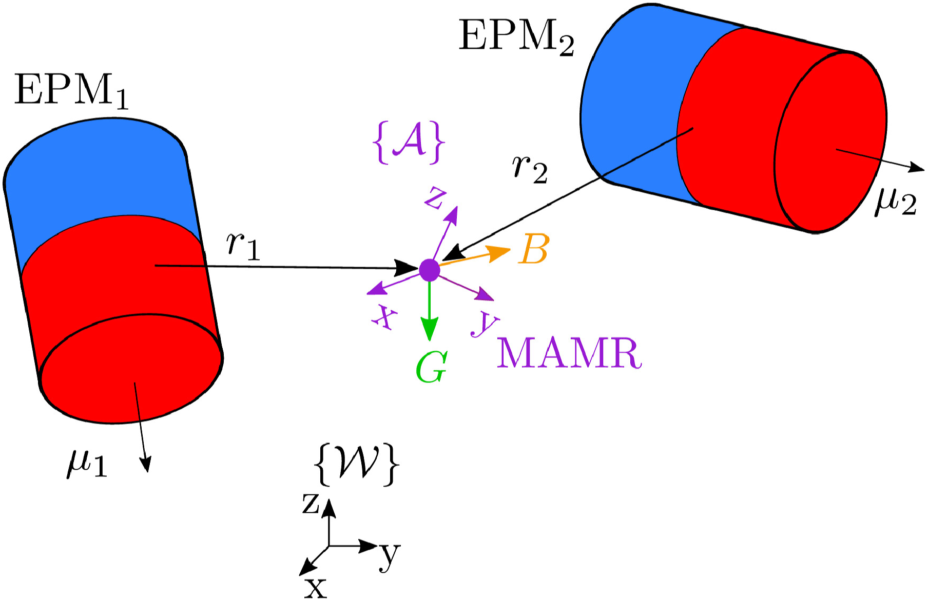 $\mathcal{W}$ } and MAMR reference frame { $\mathcal{A}$ }, together with gravity vector G in green, and magnetic field measurement B in orange.

The angular velocity measured by the gyroscope Ω can be modeled as

$\mathbf{\Omega }=\mathit{\omega }+\mathbf{b}+\mathit{\delta }$

(1)

where ω represents the MAMR’s angular velocity expressed in { $\mathcal{W}$ } relative to { $\mathcal{A}$ }, b the gyroscope bias, and δ the measurement noise.

The accelerometer measures the MAMR’s overall acceleration G and its output can be expressed as

$\mathbf{G}=R^T(\mathbf{g}+\mathbf{a})+\mathit{\sigma }$

(2)

where R denotes the rotation matrix mapping the MAMR’s orientation in { $\mathcal{W}$ }, g denotes the gravity vector in { $\mathcal{W}$ }, a the linear acceleration, and σ the measurement noise.

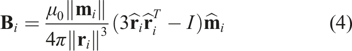
Lastly, assuming that there are no metal objects in the workspace, the magnetic field measurement B is the sum of the magnetic fields generated by each individual EPM.

$\mathbf{B}={\mathbf{B}}_1+{\mathbf{B}}_2+\mathit{\eta }$

(3)

with η denoting measurement noise. Additionally, the magnetic field generated by the ith EPM can be modeled using the dipole model (Taddese et al., 2018).

${\mathbf{B}}_i=\frac{{\mu }_0\Vert {\mathbf{m}}_i\Vert }{4\pi \Vert {\mathbf{r}}_i{\Vert }^3}(3{\widehat{\mathbf{r}}}_i{\widehat{\mathbf{r}}}_i^T-I){\widehat{\mathbf{m}}}_i$

(4)

with r _i the vector from EPM _i to { $\mathcal{A}$ }, m _i the EPM’s magnetic moment in { $\mathcal{A}$ }, and μ₀ vacuum’s magnetic permeability. We use the notation $\widehat{\cdot }=\cdot /\Vert \cdot \Vert$ , with ‖⋅‖ Euclidean norm. The dipole model has been shown to have errors lower than 2% for distances larger than 1.5 the EPM diameter (Petruska and Abbott, 2012).

In this work, we consider δ , σ , and η as zero-mean Gaussian noises, and gravity (g) dominates over linear acceleration components (i.e., a = 0) as per common approach in the literature (Mahony et al., 2008). Additionally, we assume b to be constant and offset from the measurements. Therefore, our measurement models can be written as in (1)–(3), with a = 0.

Since we assume that the zero-mean Gaussian measurement noises δ , σ , and η are not correlated with the current state, noise does not appear in the observability analysis. For the sake of investigating the system’s observability, these can be assumed zero and only the nominal (noise-free) model taken into consideration. However, the presence of noise is considered in the design of the observer, in the Extended Kalman Filter section.

2.1. Problem formulation in SE (3)

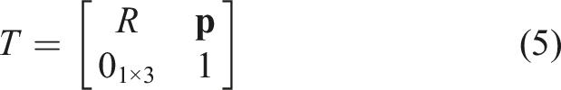
The main goal is to estimate the homogenous transformation matrix T (shown in (5)) of the MAMR’s reference frame { $\mathcal{A}$ } to the global frame { $\mathcal{W}$ }.

$T=\left[\begin{array}{cc}\hfill R\hfill & \hfill \mathbf{p}\hfill \\ \hfill 0_{1\times 3}\hfill & \hfill 1\hfill \end{array}\right]$

(5)

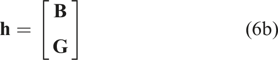
We describe our state in the special Euclidean group SE (3), where the overall system can thus be described as

$\begin{array}{l}\hfill \dot{T}=T\left[\begin{array}{cc}\hfill {\mathbf{\Omega }}_{\times }\hfill & \hfill \mathbf{v}\hfill \\ \hfill 0_{1\times 3}\hfill & \hfill 0\hfill \end{array}\right]\end{array}$

(6a)

$\begin{array}{l}\hfill \mathbf{h}=\left[\begin{array}{c}\hfill \mathbf{B}\hfill \\ \hfill \mathbf{G}\hfill \end{array}\right]\end{array}$

(6b)

where v the MAMR’s linear velocity expressed in { $\mathcal{W}$ }, and Ω_× represents the cross-product matrix form of Ω, that is, Ω_×≔(Ω × e₁, Ω × e₂, Ω × e₃), with e _i the ith element of the canonical basis of R³ (Pittiglio et al., 2020).

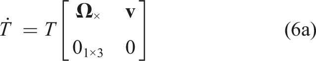
To predict the stability and performance of the observer, the observability of the system in equations (6a) and (6b) was analyzed.

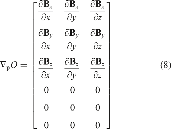
Local weak observability of a non-linear system is defined by its observability co-distribution being full rank, that is rank (∇ _T O) = 6 for this case (Pittiglio et al., 2020). In this work, we only consider the first-order derivative, and so the system’s co-distribution can be represented as

${\nabla }_{T}O=\left[\begin{array}{cc}\hfill {\nabla }_{\mathbf{p}}O\hfill & \hfill {\nabla }_{R}O\hfill \end{array}\right]$

(7)

where ∇ _p O refers to the co-distribution with respect to the position, and ∇ _R O the co-distribution with respect to the orientation.

The position co-distribution can be expanded into

${\nabla }_{\mathbf{p}}O=\left[\begin{array}{ccc}\hfill \frac{\partial {\mathbf{B}}_x}{\partial x}\hfill & \hfill \frac{\partial {\mathbf{B}}_x}{\partial y}\hfill & \hfill \frac{\partial {\mathbf{B}}_x}{\partial z}\hfill \\ \hfill \frac{\partial {\mathbf{B}}_y}{\partial x}\hfill & \hfill \frac{\partial {\mathbf{B}}_y}{\partial y}\hfill & \hfill \frac{\partial {\mathbf{B}}_y}{\partial z}\hfill \\ \hfill \frac{\partial {\mathbf{B}}_z}{\partial x}\hfill & \hfill \frac{\partial {\mathbf{B}}_z}{\partial y}\hfill & \hfill \frac{\partial {\mathbf{B}}_z}{\partial z}\hfill \\ \hfill 0\hfill & \hfill 0\hfill & \hfill 0\hfill \\ \hfill 0\hfill & \hfill 0\hfill & \hfill 0\hfill \\ \hfill 0\hfill & \hfill 0\hfill & \hfill 0\hfill \end{array}\right]$

(8)

as only the magnetic field measurements are able to provide information regarding the MAMR’s position.

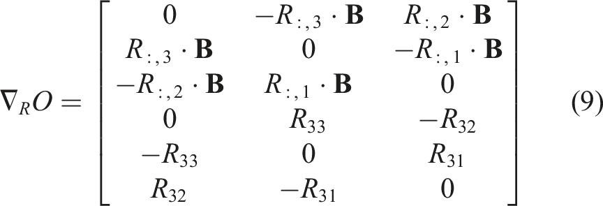
The orientation co-distribution can be expanded into

${\nabla }_{R}O=\left[\begin{array}{ccc}\hfill 0\hfill & \hfill -R_{:,3}\cdot \mathbf{B}\hfill & \hfill R_{:,2}\cdot \mathbf{B}\hfill \\ \hfill R_{:,3}\cdot \mathbf{B}\hfill & \hfill 0\hfill & \hfill -R_{:,1}\cdot \mathbf{B}\hfill \\ \hfill -R_{:,2}\cdot \mathbf{B}\hfill & \hfill R_{:,1}\cdot \mathbf{B}\hfill & \hfill 0\hfill \\ \hfill 0\hfill & \hfill R_{33}\hfill & \hfill -R_{32}\hfill \\ \hfill -R_{33}\hfill & \hfill 0\hfill & \hfill R_{31}\hfill \\ \hfill R_{32}\hfill & \hfill -R_{31}\hfill & \hfill 0\hfill \end{array}\right]$

(9)

where R_:,i denotes the ith column of matrix R. In this case, both gravity and magnetic field measurements provide information regarding the MAMR’s orientation. The full derivation of this matrix can be found in Pittiglio et al. (2020).

Looking at the full observability co-distribution, it can be seen that rank (∇ _T O) = 5, and hence the system is not observable. This can be intuitively inferred, as the gravity vector only provides information on two modes of orientation, missing the rotation around gravity. This leaves a single measurement of the magnetic field to solve for the missing four state modes, that is, position and rotation around gravity.

This is a known and common conundrum in orientation estimation in environments where the Earth’s magnetic field is not available. In previous works, multiple measurements of different magnetic field sources or at different time steps were used (da Veiga et al., 2023; Sperry et al., 2022; Taddese et al., 2018). However, these methods are either not compatible with real-time and simultaneous actuation and localization, or with multiple EPM systems. Consequently, it is helpful to split the problem into two sub-problems: the estimation of the rotation matrix in SO(3) and the estimation of the position in ${\mathbb{R}}^3$ .

2.2. Problem formulation in SO(3)

The goal here is to estimate the full rotation matrix of the MAMR R in { $\mathcal{W}$ }. This state is described in the special orthogonal group SO(3), where

$SO(3)=\{R\in {\mathbb{R}}^{3\times 3}|R^{T}R=I,\text{det}(R)=1\}$

(10)

where $I\in {\mathbb{R}}^{3\times 3}$ is the identity matrix.

Since magnetic field measurements depend on both the MAMR’s position and orientation, orientation will be estimated solely based on the accelerometer and gyroscope measurements. An observer previously described in (Pittiglio et al., 2020) is applied and can be described as follows.

$\begin{array}{l}\hfill \dot{R}=R{(\mathit{\omega }+\mathbf{b})}_{\times }\end{array}$

(11a)

$\begin{array}{l}\hfill {\mathbf{h}}_R=\left[\begin{array}{c}\hfill R^T\mathbf{g}\hfill \\ \hfill -{\mathit{\omega }}_{\times }{R}^T\mathbf{g}\hfill \end{array}\right]\end{array}$

(11b)

The state evolves over time according to the angular velocity measured from the gyroscope. The measurement model is composed by the direction of gravity measured by the accelerometer and its first derivative. This observer is able to accurately track the full orientation of a rigid body as long as some angular velocity is present in the system, independently of magnetic field measurements (Pittiglio et al., 2020). Its full derivation can be found in Pittiglio et al. (2020). Due to the single inertial measurement present, the system requires accurate initialization of the rotation around gravity. This can be achieved by calibration procedures such as the one shown in section Calibration Procedure or by the method demonstrated in da Veiga et al. (2023). Furthermore, due to the gyroscope bias b, the estimate is expected to drift over time.

2.3. Problem formulation in ${\mathbb{R}}^3$

Assuming the rotation matrix within the workspace is known through inertial sensing, the main goal is now to find the MAMR’s position $\mathbf{p}\in {\mathbb{R}}^3$ in { $\mathcal{W}$ }. For the estimation of position, only magnetic field measurements are used as IMU measurements do not depend on the position within the workspace. This system is described in equations (12a) and (12b). The observability co-distribution for the system is full-rank making the system observable.

$\begin{array}{l}\hfill \dot{\mathbf{p}}=\mathbf{v}\end{array}$

(12a)

$\begin{array}{l}\hfill {\mathbf{h}}_{\mathbf{p}}=\left[\begin{array}{c}\hfill {\mathbf{B}}_1(\mathbf{p})+{\mathbf{B}}_2(\mathbf{p})\hfill \end{array}\right]\end{array}$

(12b)

As shown previously (da Veiga et al., 2023), the relative pose of the EPMs highly affects the system’s observability and the observer’s performance. As such, Figure 2 depicts the system’s condition number across the workspace for the most common EPM configurations of the platform (Pittiglio et al., 2022a). The condition number is defined as the ratio between the maximum and minimum singular values of the systems observability co-distribution matrix (Taddese et al., 2018), and therefore, lower values indicate a better conditioned system. We can see that singularity planes and regions exist for certain configurations as shown by a high condition number. These singularity planes are characterized by unidirectional magnetic fields. Figure 3 plots the magnitude of the magnetic field on these planes. For brevity, the singularity planes for the EPM configurations when the EPMs are magnetized along Z (Figure 2(c) and (g)) were omitted as they are identical to magnetizations along X (Figure 2(a) and (e)) albeit rotated by 90° around the y axis.

Figure 2.

Position estimation in ${\mathbb{R}}^3$ condition number across the workspace for different relative poses between the EPMs. The configurations depicted in (a), (b), and (c) generate a homogenous field along the X, Y, and Z axis, respectively, in the workspace center. Scenarios (e), (f), and (g) generate magnetic field derivatives ∂B _x /∂y, ∂B _y /∂y, and ∂B _z /∂x, respectively, in the workspace center. Configurations (d) and (h) represent orthogonal configurations of the EPMs magnetic moments.

Figure 3.

Field magnitude on singularity planes for different EPM configurations. The magnetic field on these planes is unidirectional and orthogonal to the plane, each line denoting a magnitude. (a) Homogenous field along the X axis, (b) homogenous field along the Y axis, and (c) and (d) magnetic field gradient ∂B _x /∂y.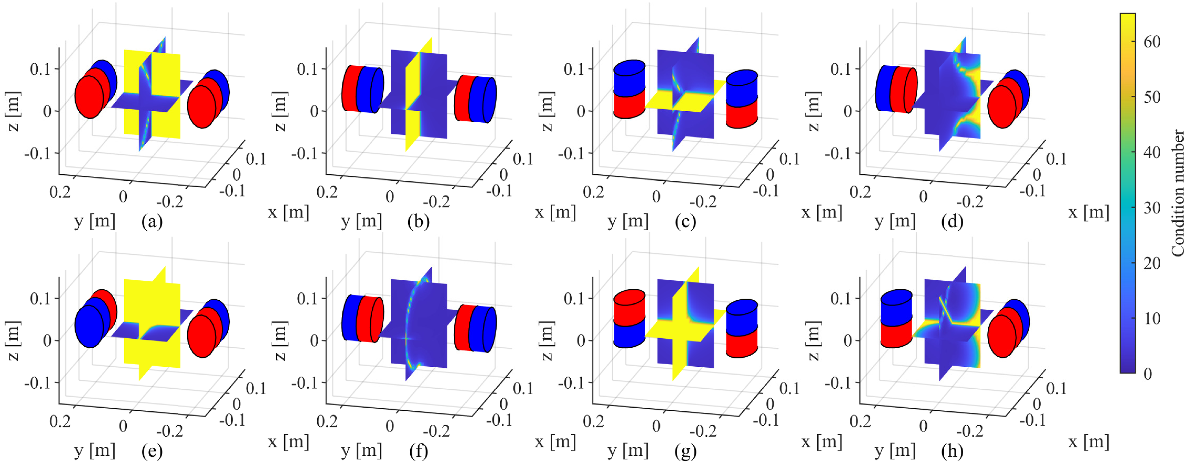

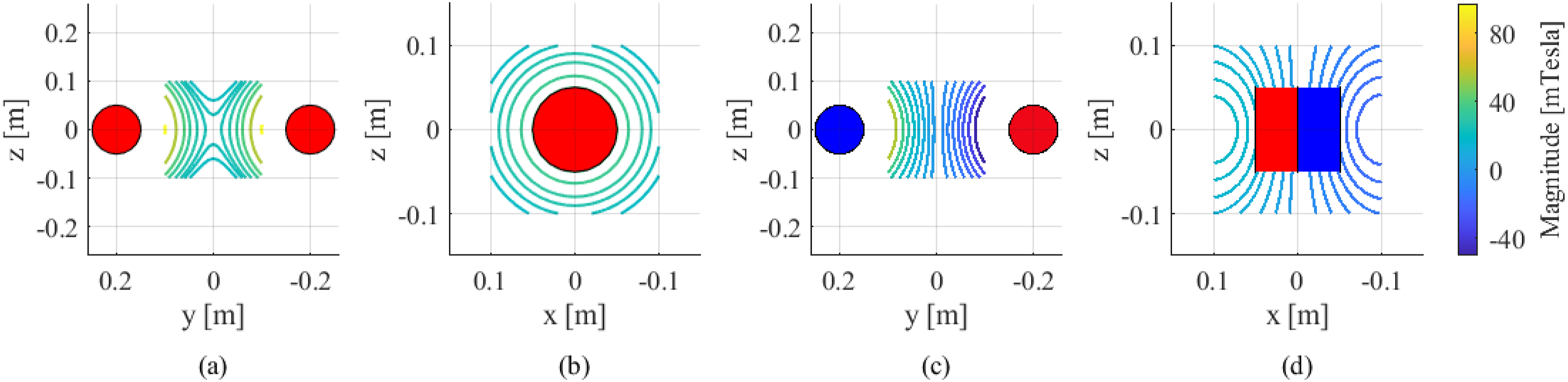
It is known that for a single cylindrical axially-magnetized EPM, the plane orthogonal to its magnetization passing through its center is singular (Taddese et al., 2018). This plane is characterized by magnetic fields which are perfectly aligned with the magnetization of the PM. These are symmetric concentrically around the PM, and thus an infinite number of points have the exact same magnetic field vector. This effect is replicated on the plane equidistant from two EPMs when these are perfectly aligned along their magnetizations (Figures 2(b) and 3(b)).

When two EPMs are parallel to each other (Figures 2(a) and (c), and 3(a)), the single EPM singularity plane is still singular as the magnetic field on that plane is uniaxial and concentrically symmetric, although around two centers rather than one. Additionally, when the EPMs are parallel with their magnetizations opposed (Figure 2(e) and (g)), a second singularity plane is present (Figure 3(c) and (d)), as the magnetic field is also unidirectional and symmetric on the equidistant plane between the two EPMs.

These singularity planes can be mitigated by having the EPMs misaligned (Figure 2(d) and (h)), where only small singularity regions are present closer to each EPM singularity plane.

2.4. Observer simulation

In order to evaluate the feasibility of the proposed method, we implemented a simulated observer. The results can be seen in Figure 4. For the purpose of this simulation, the observer runs at 200 Hz and the MAMR moves with a maximum linear velocity of 5 mm/s and maximum angular velocity of 5° per second. As we can see, the observer successfully tracks both the position and orientation, converging to the right position estimate in under 5 s. The effect the EPMs singularity conditions have on the convergence of the observer is explored in Section Singularity Conditions, and the effect the gyroscope bias has on the orientation estimate is explored in Section Random Continuous Movement. Both of these are explored with experimental data to accurately represent real-world conditions.

Figure 4.

Simulated observer showing the estimated state in full lines and ground truth in dashed lines for both position (a) and orientation (b).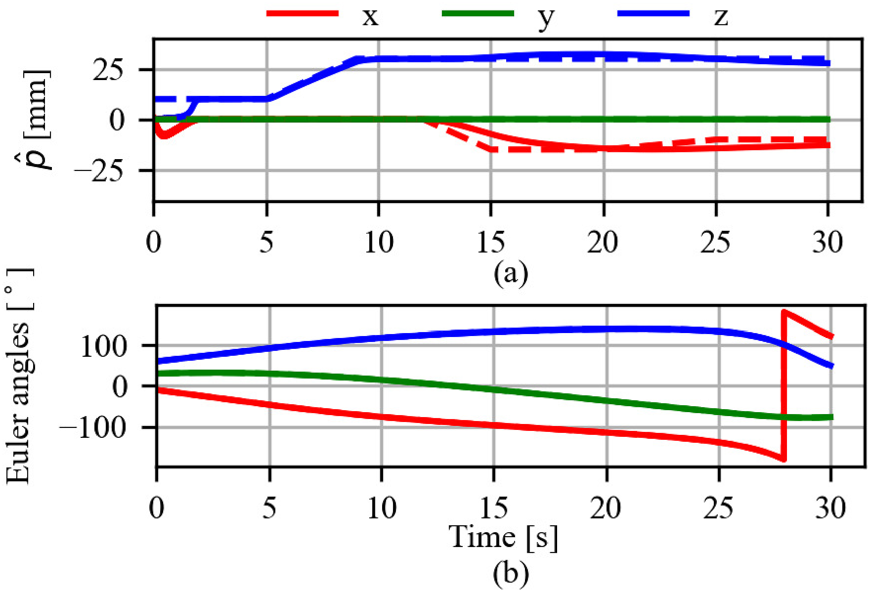

3. Experimental setup

The proposed localization technique was evaluated on a magnetically actuated soft continuum robot (SCR), under dEPM actuation.

3.1. Soft continuum robot

The SCR featured a sensorized tip containing a 3D HE and an IMU. Figure 5 depicts a schematic representation of the fabrication process. Silicone rubber (Ecoflex®00-30, Smooth-On, Inc., U.S.A.) was mixed with hard magnetic micro-particles (NdFeB with an average 5 μm diameter and intrinsic coercivity of H _ci = 9.65 kOe, MQFP-B+, Magnequench GmnH, Germany) in a 1:1 weight ratio. The mixture was mixed and degassed in a high-vacuum mixer (ARV-310, THINKYMIXER, Japan) for 90 s at 1400 rpm and 20.0 kPa (da Veiga et al., 2021). The elastomer was subsequently injected into a 3D printed mold and left to cure at room temperature (Figure 5(a)). Once cured, the SCR was magnetized under a magnetizing field of 5.0 T using an impulse magnetizer (IM-10-30, ASC Scientific, U.S.A).

Figure 5.

Schematic representation of the continuum robot fabrication with a sensorized tip containing an IMU and HE sensor. (a) Silicone rubber with magnetic particles is injected into a mold. (b) Sensors are held in place through a PCB holder which is embedded in the overall SCR.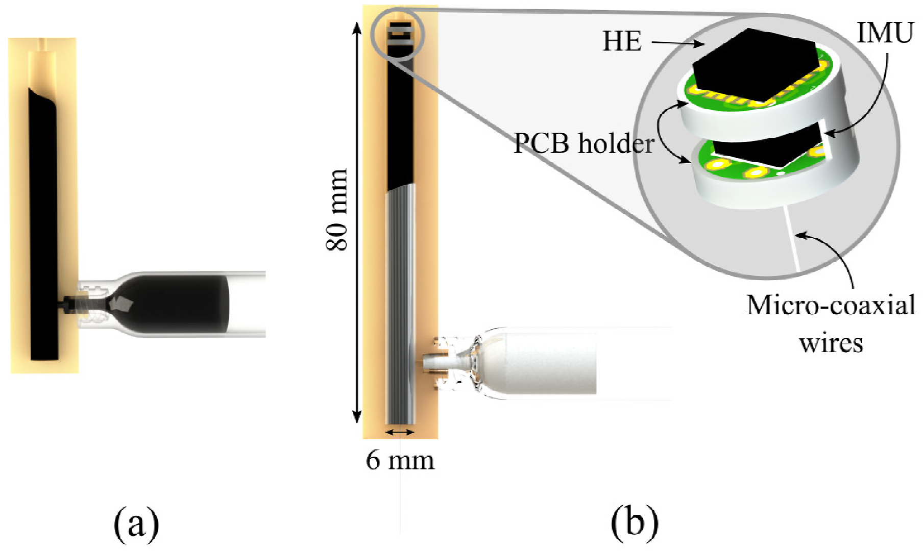

Separately, the sensors were soldered onto 5 mm diameter circular printed circuit boards (PCBs), and then fitted into a 3D printed holder (with an outer diameter of 5.5 mm). The sensors used were chosen due to their dimensions, sensitivity and sensing range, allowing their use in small embedded devices under high magnetic fields (IMU: LSM6DS3, STMicroelectronics, Switzerland. Accelerometer sensing range ±16 g, Sensitivity 0.488 mg/LSB₁₆; Gyroscope sensing range ±2000 mdps, sensitivity 70 mdps/LSB₁₆; Hall Effect: MLX90395, Melexis, Belgium. Sensing range ±50 mT; Sensitivity 2.5 μT/LSB₁₆). This was then placed at the distal end of a second 3D printed mold together with the SCR, and then non-magnetic silicone elastomer was injected (Figure 5(b)). The final SCR was 6 mm in diameter, and 80 mm in length, with an axial magnetization.

3.2. Sensor calibration

Once the SCR was fabricated, the sensors were calibrated. This calibration has the main goal of finding the orientation of the ICs inside the SCR. The accelerometer was calibrated by measuring gravity along the SCR inertial axes. The gyroscope was offset by measuring its output for 10 min while stationary. The HE sensor was calibrated by placing the SCR tip in the center of a Helmholtz coil (DXHC10-200, Dexing Magnet Tech. Co., Ltd, Xiamen, China) under known homogeneous magnetic fields. The sensors were interfaced to a Raspberry Pi 4B through i²c protocol.

Given that the SCR is magnetic, its effect on the measurement of the external magnetic field has to be considered. To this effect, the magnetic field measurements were offset by measuring the internal magnetic field when the SCR is under no external actuation, which was equal to 3.2 mT (see Figure 6(a)). Furthermore, unlike traditional rigid magnetic robots where the internal magnet is rigidly affixed with respect to the internal sensors, in SCR their relative position changes with deflection. This can influence the internal-magnetic field offset. This being so, the SCR was then actuated under a known external magnetic field of 9 mT in a Helmholtz coil (DXHC10-200, Dexing Magnet Tech. Co., Ltd, Xiamen, China) (see Figure 6(b)) where the internal magnetic field measured was of 3.1 mT. Given these results, in this work, the internal magnetic field to the SCR is considered constant.

Figure 6.

Fabricated Soft Continuum Robot (a) unactuated and (b) under a 9 mT homogeneous magnetic field.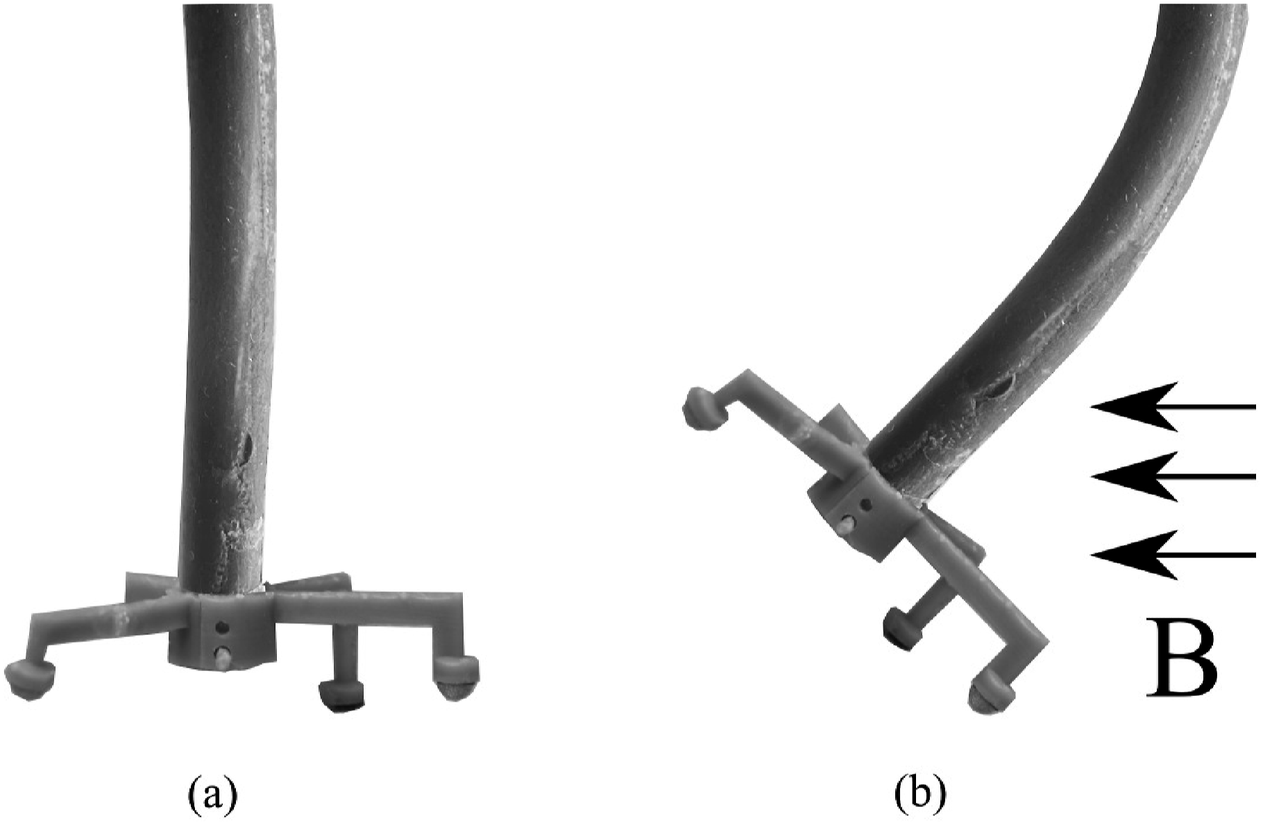

3.3. Dual external permanent magnet platform

The dEPM platform was used to test the localization technique (Pittiglio et al., 2022a). This platform is comprised of two KUKUA LBR iiwa14 robots (KUKA, Germany), each manipulating one EPM (cylindrical permanent magnet with diameter and length of 101.6 mm and axial magnetization of 970.1 Am² (Grade N52)) (see Figure 7). The platform is able to generate magnetic fields up to 50 mT and magnetic field gradients of up to 300 mT/m at the center of the workspace. The SCR was placed in the center of the workspace with its base fixed in place at the origin, and its tip free to move.

Figure 7.

Experimental setup for the localization experiments. In orange is the optical tracker used as benchmark data. In red the PCBs with the embedded sensors.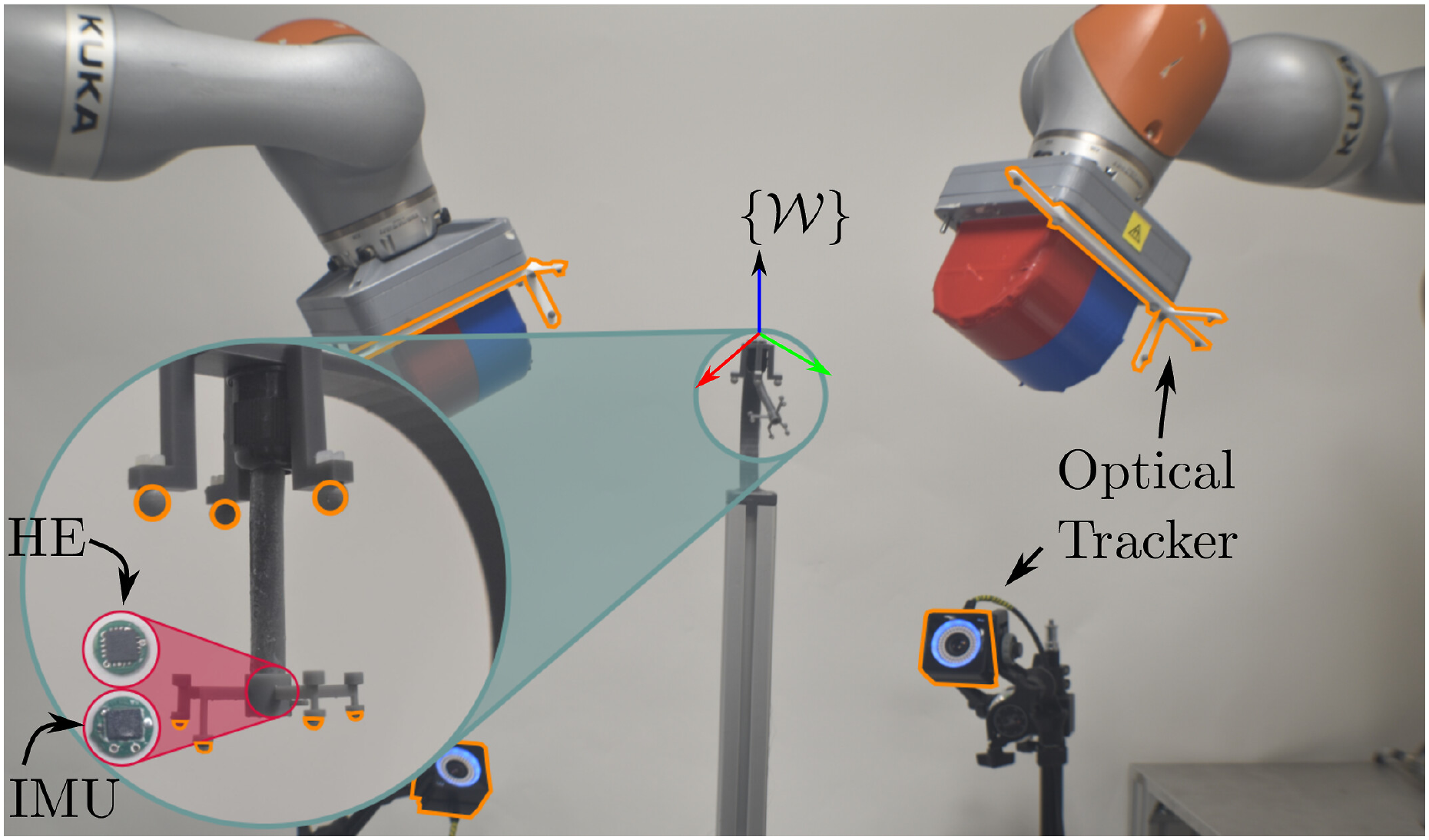

Additionally, a 4-camera optical tracking system (OptiTrack, Prime 13, NaturalPoint, Inc., U.S.A., with submilimeter accuracy) was used for ground truth measurements. Markers were attached to the end-effectors of both robots, the workspace center and the SCR tip. Robot Operating System (ROS) was used to operate the robotic arms and to read data from sensors at 300 Hz.

3.4. Extended Kalman filter

The Extended Kalman Filter (EKF) has been proved effective in localization techniques (Pittiglio et al., 2020). Here, we describe the discrete-time dynamics of the position, followed by the prediction and update steps of the EKF. For the sake of summary, we present the general form of the EKF, which was applied to estimate the orientation and the position separately.

3.4.1. Orientation discrete dynamics

The discrete dynamics of the estimated orientation $\widehat{R}$ can be described as

$\begin{array}{l}\hfill {\widehat{R}}_{k+1}={\widehat{R}}_k\text{exp}({\mathit{\omega }}_{k_{\times }})\text{exp}({(K_k{\tilde{\mathbf{z}}}_k)}_{\times })\end{array}$

(13a)

$\begin{array}{l}\hfill {\tilde{\mathbf{z}}}_k={\mathbf{z}}_k-{\mathbf{h}}_R({\widehat{R}}_k,{\mathit{\omega }}_k)\end{array}$

(13b)

with k = 0, T, 2T, … and K _k the Kalman gain defined below, exp (⋅) denotes the exponential map of SO(3), z _k the output from the IMU, and h _R (⋅) the measurement model proposed in equation (11b).

3.4.2. Position discrete dynamics

The estimated position $\widehat{\mathbf{p}}$ discrete dynamics are described as follows

$\begin{array}{l}\hfill {\widehat{\mathbf{p}}}_{k+1}={\widehat{\mathbf{p}}}_k+K_k{\tilde{\mathbf{z}}}_k\end{array}$

(14a)

$\begin{array}{l}\hfill {\tilde{\mathbf{z}}}_k={\mathbf{z}}_k-{\mathbf{h}}_{\mathbf{p}}({\widehat{\mathbf{p}}}_k)\end{array}$

(14b)

with z _k the output from the HE sensor, and h _p (⋅) the measurement model proposed in equations (12a) and (12b).

3.4.3. EKF prediction step

The prediction step of the EKF consists of propagating the state covariance P _k as

$P_k=F_k{\overline{P}}_{k-1}{F}_k^T+Q_n$

(15)

where F _k denotes the state derivative of the system dynamics, G _k the state derivative of the measurement model, and Q _n the input noise covariance matrix.

3.4.4. EKF update step

The update step computes the Kalman gain according to the following equations.

$S_k=H_k{P}_k{H}_k^T+N_n$

$K_k=P_k{H}_k^T{S}_k^{-1}$

${\overline{P}}_k=P_k-K_k{S}_k{K}_k^T$

with N _n the measurement noise covariance matrix.

3.5. Error metrics

Each observer’s performance was assessed through the norm of the error. For the position observer, the norm was computed as shown in equation (16).

$\Vert \tilde{\mathbf{p}}\Vert =\Vert \mathbf{p}-\widehat{\mathbf{p}}\Vert$

(16)

For the orientation observer, the error of the whole rotation matrix was computed through equation (17).

$e_R=\text{tr}(I-{\widehat{R}}^{T}R)$

(17)

Unlike position, orientation is a bounded entity with a maximum error, e _R ∈ [0, 4]. Therefore, the orientation errors are expressed as a percentage.

4. Platform calibration

In order to estimate the SCR’s pose within the workspace, the global reference frame first needs to be defined. Unlike single EPM in which the localization focuses on finding the relative pose between the MAMR and the EPM, or coil-based platforms where the global reference frame is well defined due to the platform’s static nature, when two or more EPMs are present, the localization is done with respect to a previously defined global reference frame. Therefore, this calibration procedure aims at defining such a frame and finding the relative transformation matrices of both robotic arms ( $T_{{\mathcal{B}}_1}^{\mathcal{W}}$ and $T_{{\mathcal{B}}_2}^{\mathcal{W}}$ ). This was previously done through an optical tracking system (da Veiga et al., 2023; Pittiglio et al., 2022a, 2022b). However, the requirement of additional equipment and free line of sight between the cameras and markers are not ideal in a clinical environment, and can severely limit the accuracy of results.

In this work, we propose a viable alternative through magnetic localization. By fixing a magnetic field sensor with reference frame $\mathcal{S}$ in the workspace, and taking its pose as the new workspace origin $\mathcal{S}=\mathcal{W}$ , this sensor can be localized with respect to each robotic arm one at a time $T_W^{{\mathcal{B}}_1}$ and $T_W^{{\mathcal{B}}_2}$ . This sensor can be embedded in a device which is not responsive to magnetic fields, or be embedded in a magnetically actuated device and ensuring these calibration fields are low in intensity. From here on we describe the methodology for a generic robotic arm, repeating the process for every robotic arm present in the system. This calibration procedure needs to be done every time the relative pose between the robotic arms’ bases changes, for example when an alternative arrangement between robotic arms is needed.

4.1. Observer

For the calibration of the dEPM we consider only magnetic field measurements and no IMU. This limits the required hardware for the calibration procedure. The goal is to find the relative pose between the sensor and the base of the robotic arm $T_W^{\mathcal{B}}$ . The homogenous transformation between the robotic arm base and the EPM is assumed to be known and read from the robotic arm encoders. Since only magnetic field measurements are available, the calibration process focuses first on finding the position of the sensor, followed by its orientation.

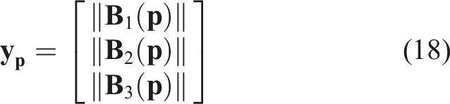
The position is first estimated by using the measurement model described in equation (18). It is composed of three separate measurements of the magnetic field norm for three different EPM positions.

${\mathbf{y}}_{\mathbf{p}}=\left[\begin{array}{c}\hfill \Vert {\mathbf{B}}_1(\mathbf{p})\Vert \hfill \\ \hfill \Vert {\mathbf{B}}_2(\mathbf{p})\Vert \hfill \\ \hfill \Vert {\mathbf{B}}_3(\mathbf{p})\Vert \hfill \end{array}\right]$

(18)

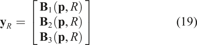
Once the position is estimated, the orientation is subsequently estimated offline, using the same set of measurements but using the magnetic field vector, since its position p is now known.

${\mathbf{y}}_R=\left[\begin{array}{c}\hfill {\mathbf{B}}_1(\mathbf{p},R)\hfill \\ \hfill {\mathbf{B}}_2(\mathbf{p},R)\hfill \\ \hfill {\mathbf{B}}_3(\mathbf{p},R)\hfill \end{array}\right]$

(19)

This allows the estimation of the full 6-DOF pose of a static magnetic field sensor where the EPM movements are not used for actuation and purely for localization.

4.2. EPM path

The path the EPM travels has a significant impact on the estimation error across the workspace. Ideally, for the calibration of the system the path should cover as much of the workspace as possible and generate significantly different measurements in order to provide as much information as possible. However, such a path is difficult to achieve in a short amount of time and space. For this reason, four different EPM paths were simulated and the position across the workspace estimated. These paths were generated to cover a wide range of EPM positions, EPM motion directions, and variations of magnetic field produced. For all simulated paths, the EPM was constrained to stay in a single side of the workspace, and all paths had the same number of points, taking between 200 and 300 s to complete, assuming a safe EPM speed (30% of maximum speed of the robotic arm, 4 cm/s).

Figure 8 shows the results obtained for the position estimation across the workspace for each path tested. The paths tested were: four planar circles (Figure 8(a)), four circles in different planes (Figure 8(b)), spiral planar motion (Figure 8(c)), and a random planar path (Figure 8(d)). As we can see for all cases, the majority of the workspace is estimated with errors lower than 5 mm. The random movement (Figure 8(d)), despite having the highest level of variety of movement, leads to several points of high error, especially closer to the EPM. The spiral movement (Figure 8(c)), overall, was the trajectory with the lowest number of points with higher error, and these were concentrated on one of the corners of the workspace. For this reason, this was the path chosen for testing.

Figure 8.

Simulated EPM paths (in black) and corresponding error norm for estimation of the position across the workspace, for the calibration of the system. (a) Four circles on plane y = −0.2; (b) four circles across planes y = −0.2, x = 0, and z = 0;(c) spiral on plane y = −0.2; (d) random path with boundaries −0.2 < x, z < 0.2 and −0.25 < y < − 0.2.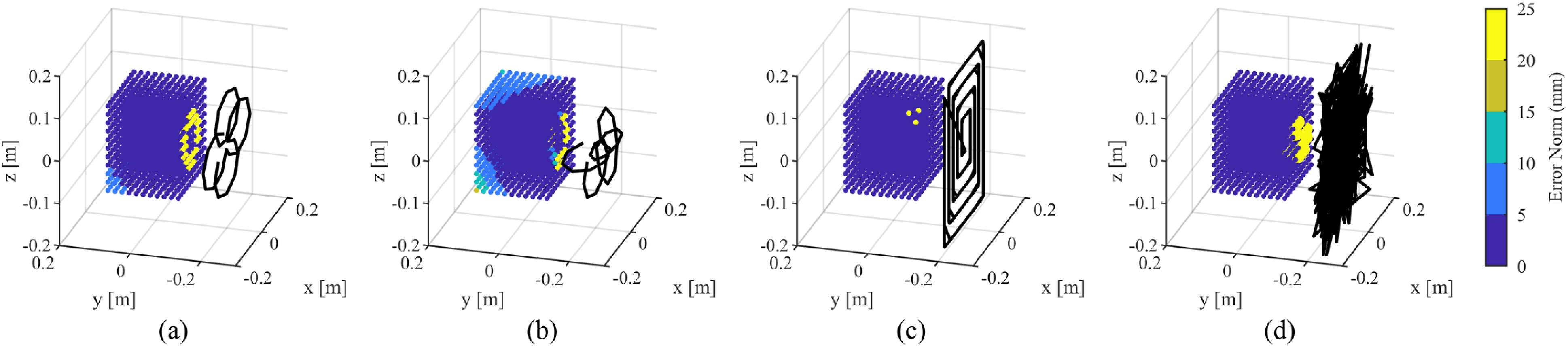

4.3. Experimental setup

For the calibration procedure a 3D printed plate with the HE sensor in multiple configurations was placed in the center of the workspace (Figure 9). Optical tracker markers were attached to both the plate and the sensor for ground truth measurements. Both robotic arms were moved away from the workspace until no magnetic field measurements were present. Each arm was then brought into the workspace, one at a time, for calibration.

Figure 9.

Experimental setup for the calibration of the platform. The optical tracker used as benchmark is outlined in orange, and the HE sensor in pink.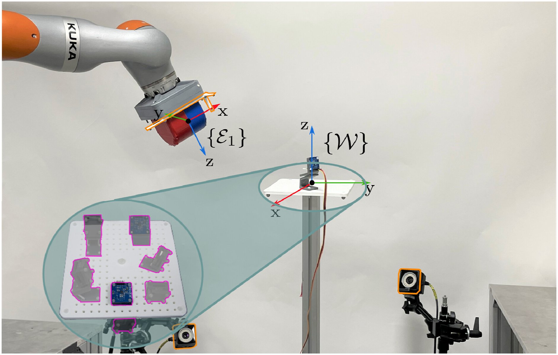

4.4. Results

The EKF parameters for the position estimation were P_P0 = diag(10I), Q _Pk = diag(0.1I) and R _P = diag(0.1I), with $I\in {\mathbb{R}}^{3\times 3}$ the identity matrix. The EKF parameters for the orientation were P_R0 = diag(1I), Q _Rk = diag(10I) and R _R = diag(0.001I). The position estimate was initialized at the workspace center, and the orientation as the identity matrix. The EPM was moved along a spiral path covering a wide area of the workspace taking 250 s. Seven different poses within the workspace were tested (Figure 10(a)). The results for the calibration step are shown in Figure 10(b).

Figure 10.

Results for calibration procedure. (a) Workspace containing the seven tested points together with the spiral path traveled by the EPM. (b) Error norm in position and orientation for each point versus the EPM path.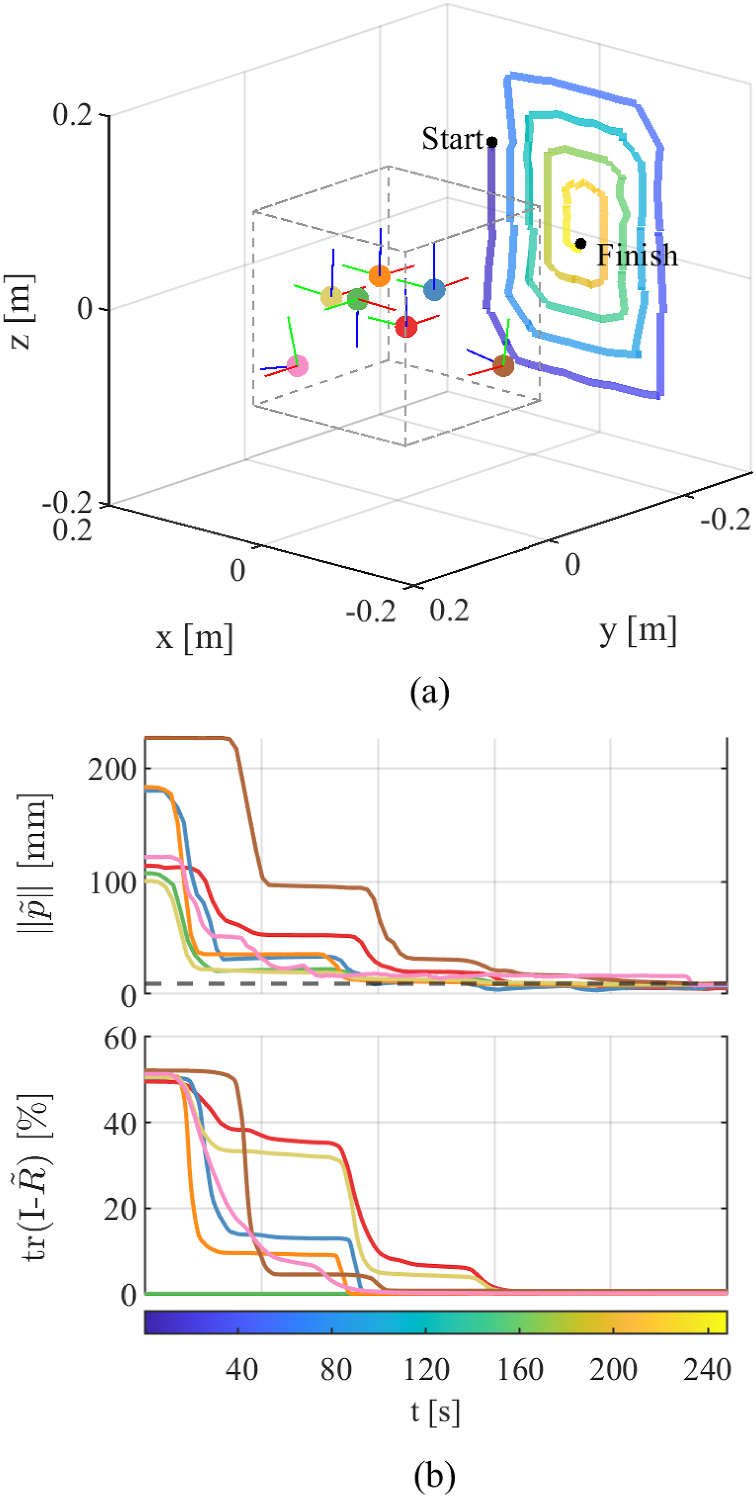

The average error in position norm was 5.3 ± 1.8 mm, with 2.4 ± 1.4 mm along the x axis, 2.9 ± 1.7 mm along y, and 2.8 ± 1.4 mm along z. The final orientation percentage error was 0.14%, with 1.5 ± 1.3° in x, 1.9 ± 1.4° in y, and 3.5 ± 3.7° in z.

5. Pose estimation

Once the platform has been calibrated and the poses of the two robotic arms in the global reference frame are known, the SCR can be actuated and localized. The EKF parameters for the estimation of both the orientation and position as described previously can be found in Table 1. Additionally, as stated earlier the orientation observer needs to be initialized with an accurate estimate R₀. In this work, this was found using the benchmark data. In a clinical realistic environment, this could be found using static localization methods (da Veiga et al., 2023), or by inserting the SCR from a known pose. The position observer was initialized at the center of the workspace.

Table 1.

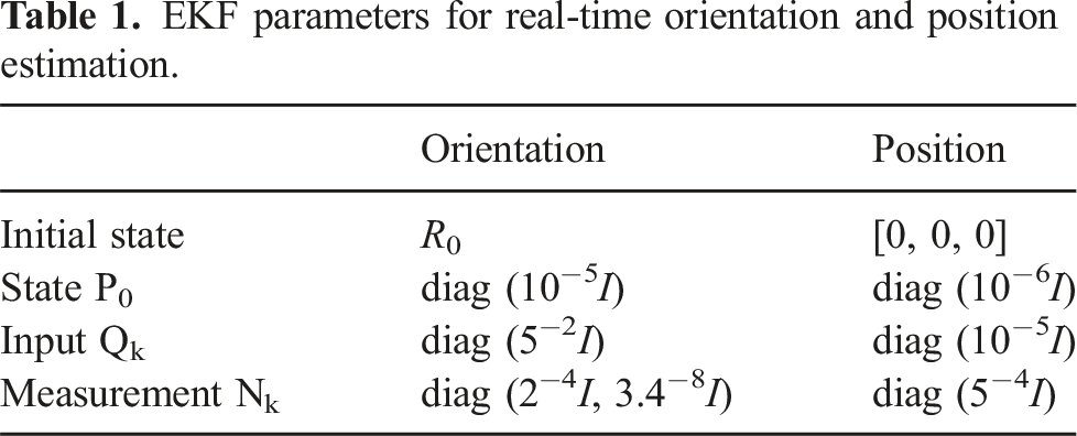
EKF parameters for real-time orientation and position estimation.

	Orientation	Position
Initial state	R 0	[0, 0, 0]
State P0	diag (10−5I)	diag (10−6I)
Input Qk	diag (5−2I)	diag (10−5I)
Measurement Nk	diag (2−4I, 3.4−8I)	diag (5−4I)

5.1. Singularity conditions

As shown previously, certain configurations of the two EPMs generate singularity regions in which the estimation of the position becomes challenging. As such, alternative EPM configurations which produce the same SCR deflection and tip position need to be found in order not to lose functionality of the SCR while simultaneously avoiding singularity conditions. Given the high non-linearity of the magnetic fields generated by two EPMs, and the flexibility of the dEPM platform, these alternative EPM configurations can be easily achieved.

Figures 11–14 show the singularity EPM configuration and the alternative EPM configuration ((a) in green and brown, respectively) which produce the same SCR tip deflection ((b) black dot denoting starting SCR tip position), and the localization results for both cases ((c)) (see Supplemental Video 1). The system was initialized (at t = 0) with the EPMs away from the workspace, and therefore in the absence of any magnetic field measurements, and the EPMs were moved into their final positions (shown in (a)). We can see, that for the singularity conditions, the observer executed very poorly, not converging to the correct solution, with an average error in position norm of 53.1 ± 20.3 mm. Conversely, the alternative EPM configurations that produced the same SCR deflection yielded much better results, with an average error of 4.5 ± 1.8 mm (5.6% of SCR length), and converging to the right position in under 10 s. Additionally, we can see the observer was able to maintain an accurate estimate once the SCR reached stability.

Figure 11.

Movement along the positive X axis. (a) Shows the two EPM configurations; (b) the position of the continuum robot for the two EPM configurations; (c) orientation and Position error for the two EPM configurations.

Figure 12.

Movement along the negative X axis. (a) Shows the two EPM configurations; (b) the position of the continuum robot for the two EPM configurations; (c) orientation and position error for the two EPM configurations.

Figure 13.

Movement along the positive Y axis. (a) Shows the two EPM configurations; (b) the position of the continuum robot for the two EPM configurations; (c) orientation and position error for the two EPM configurations.

Figure 14.

Movement along the negative Y axis. (a) Shows the two EPM configurations; (b) the position of the continuum robot for the two EPM configurations; (c) orientation and position error for the two EPM configurations.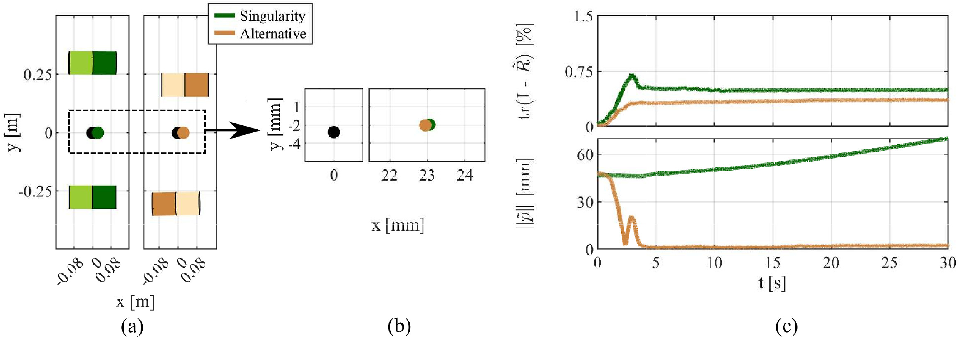

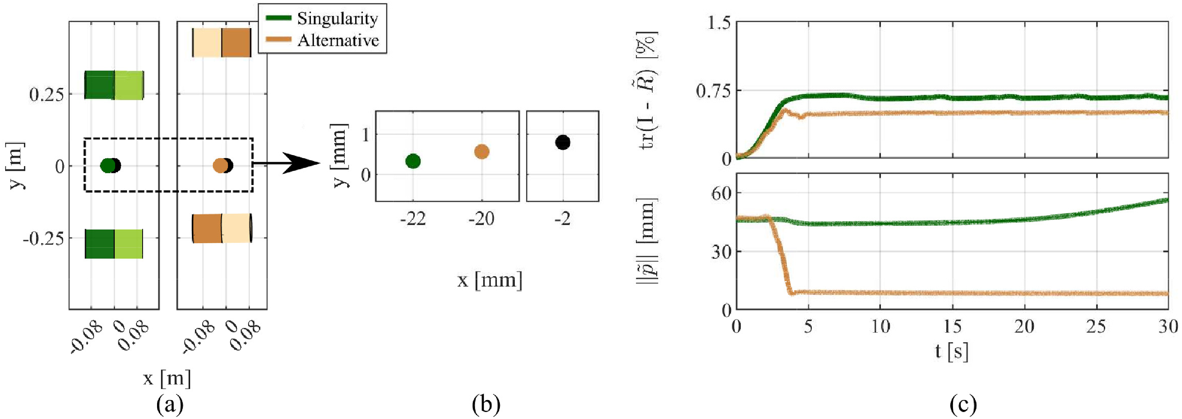
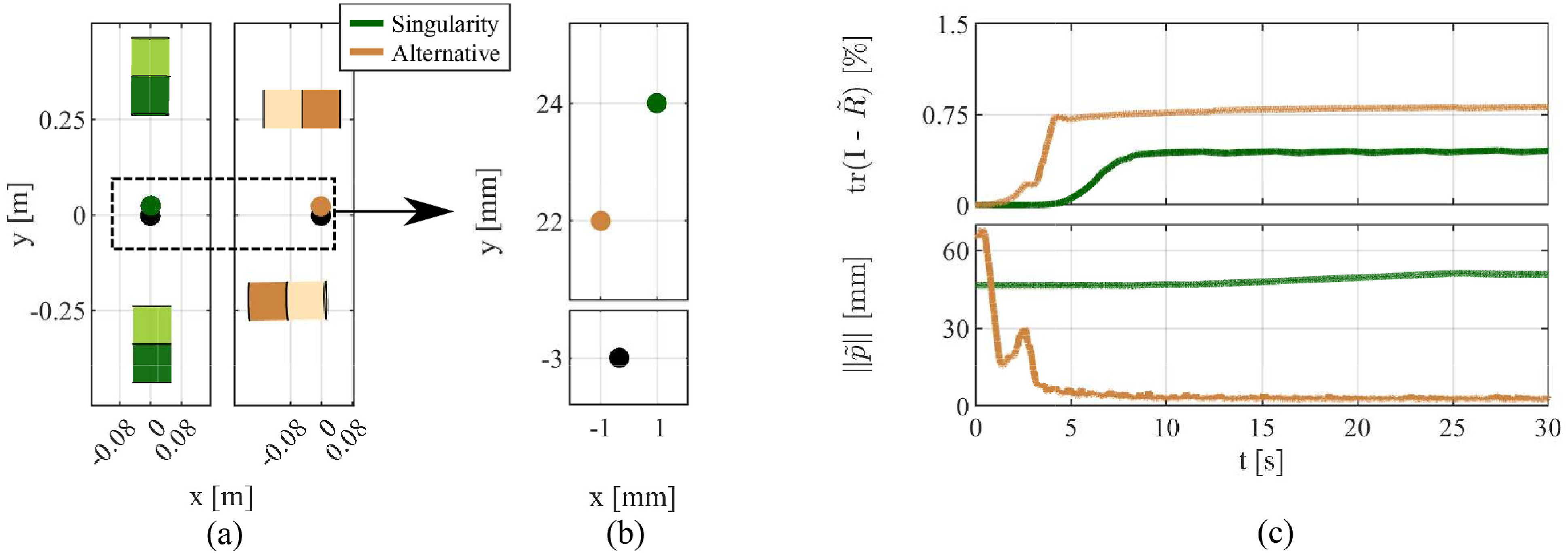
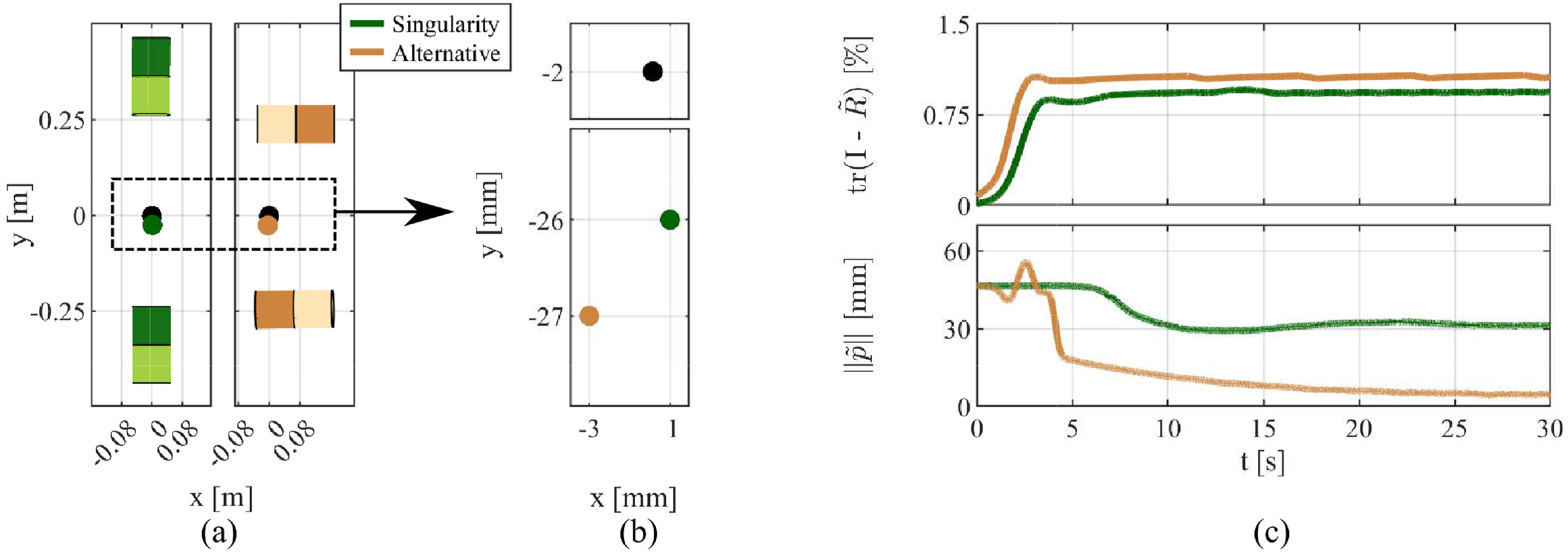
Since the orientation estimation does not depend on the magnetic field measurements, the errors in orientation were similar across all cases, with an average percentage error of 0.63%, with 1.0 ± 0.7° for x, 0.6 ± 0.5° for y, and 5.2 ± 0.2° for z.

5.2. Random continuous movement

To analyze the stability of the localization against gyroscope drift and possible momentary singularity regions, the EPMs were moved along random paths while the SCR was actuated freely for a total duration of 10.5 min. This will also test the stability of the localization against quick and large changes in pose.

Figure 15 depicts the full 6-DOF pose estimation results for random movements of the EPMs over the whole time period, together with the error over time for both the orientation and position. Additionally, an expanded view of the estimated state for the first and last minute can be found in Figure 16. The estimation for the entire duration can be seen in the Supplemental Video 2.

Figure 15.

Results for the 6-DOF localization for when the EPMs are traveling along random paths. Full lines denote the estimated state against the ground truth data (dashed lines). The estimated rotational angles (a) and the error in the estimation of the rotation matrix (b). The estimated positional values (c), and its corresponding error norm (d).

Figure 16.

Expanded view of the estimated state against ground truth data for the first ((a) and (c)) and last ((b) and (d)) minute.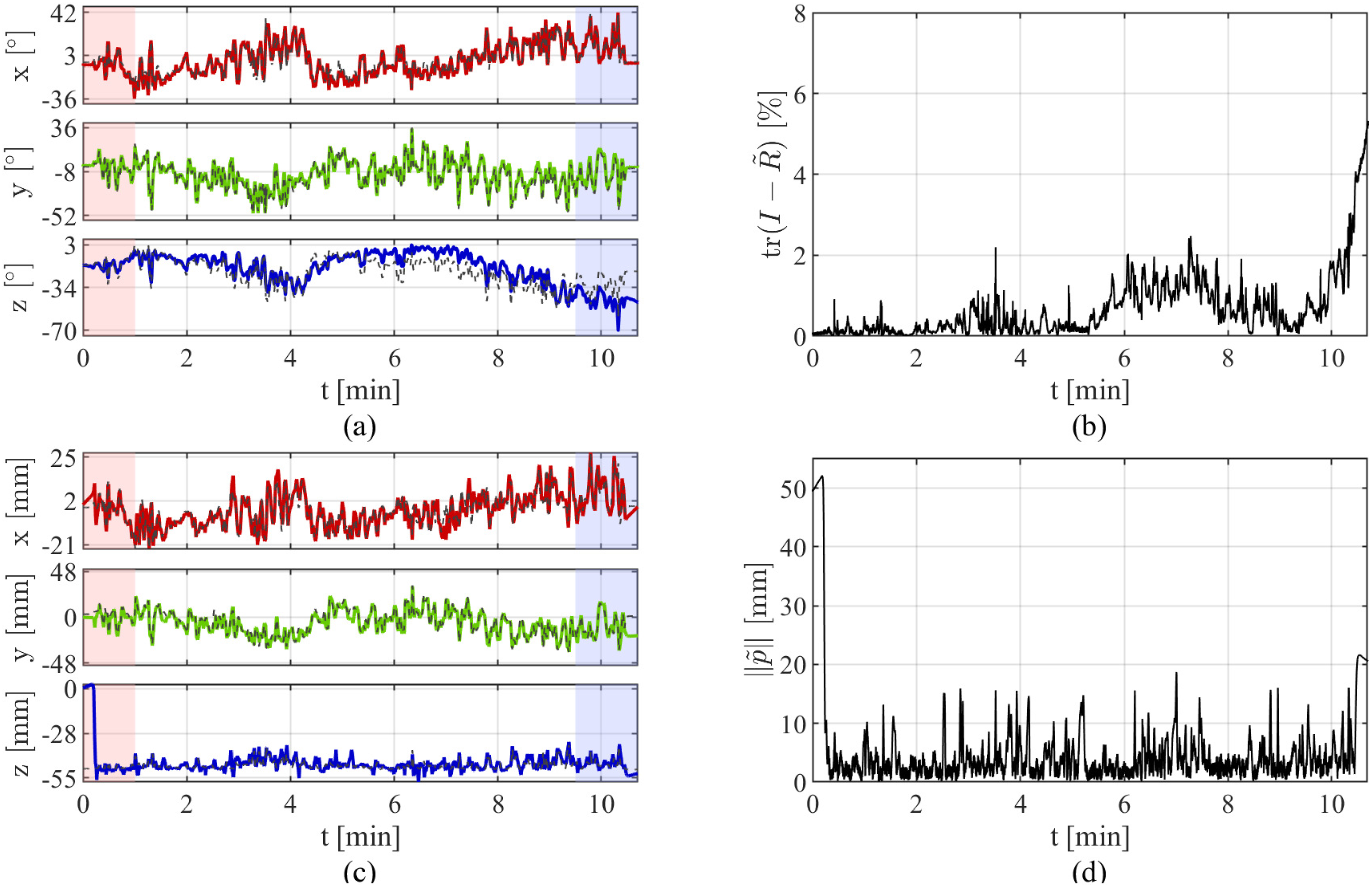

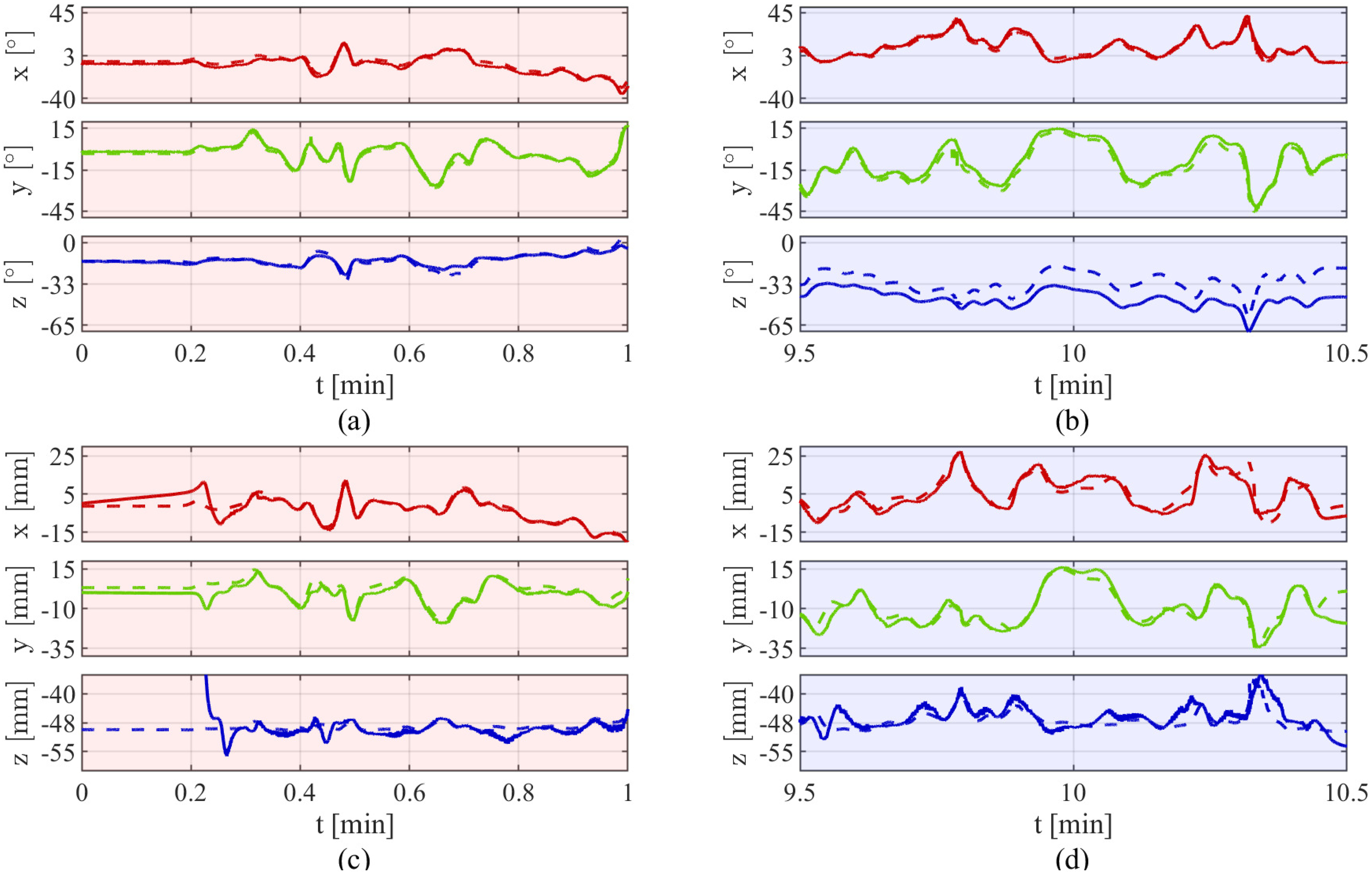
As we can see in Figure 15(b) the observer maintained orientation errors under 1% during the first half of the running time. However, this error increased toward the end, mainly due to inaccurate rotation around gravity (Figure 16(b)). This is expected since there is only a single inertial measurement present in the system, leaving the rotation around gravity to be estimated solely on the biased gyroscope output. This bias, when integrated over time, makes the estimate drift. In this work, this bias was considered constant, and that assumption was enough to maintain an accurate orientation estimate for the first 5 min, with average errors of 0.21%, the equivalent of 2.5 ± 1.6° around x, 1.5 ± 1.2° around y, and 2.8 ± 2.2° around z. However, by the end of the running time, 10 min and 30 s, the error of orientation around gravity was of 26.4° increasing the error in the orientation estimation up to 5.2%.

When looking at the position estimation, we can see that the observer converged to the right state within the first 15 s, with an average error of 3.5 ± 2.7 mm (4.3% of SCR length) in norm after convergence during the first 5 min, and of 4.1 ± 3.8 mm (5.1% of SCR length) for the full time-scale. Additionally, the error spike at the end of the time period is due to the removal of magnetic field when the EPMs are moved away from the workspace. Since the EPMs are traveling along random paths, there are moments of magnetic singularity affecting the estimate of the position. However, we can see that the observer is able to quickly re-converge to the right state. Furthermore, the position errors for the first 5 min are around 58% lower when compared to our previous work (da Veiga et al., 2023). This is due to the fact that the orientation is estimated independently of the position and magnetic field measurements. In our previous work, both the position and orientation estimates are affected by magnetic singularity regions.

5.3. Maximum error in initial state estimate

A known disadvantage of an EKF is the negative impact the initial estimate of the state may have on the observer’s convergence. As expressed in Table 1, the initial positional state was defined as the workspace origin, translating into an initial error of 4.9 cm. To evaluate the maximum initial error the observer can withstand and still converge, the localization algorithm was tested against a range of initial state errors.

Figure 17 plots the state error at 30 s for initial state errors of up to 40 cm. As it can be seen, the observer converges in less than 30 s for errors of up to 35 cm. When the error was of 40 cm the observer failed to converge. Given that in this work we assume a cubic workspace of size length of 20 cm, it is expected that the EKF will converge as long as the initial state is inside the workspace.

Figure 17.

Initial positional state error versus state error at 30 s.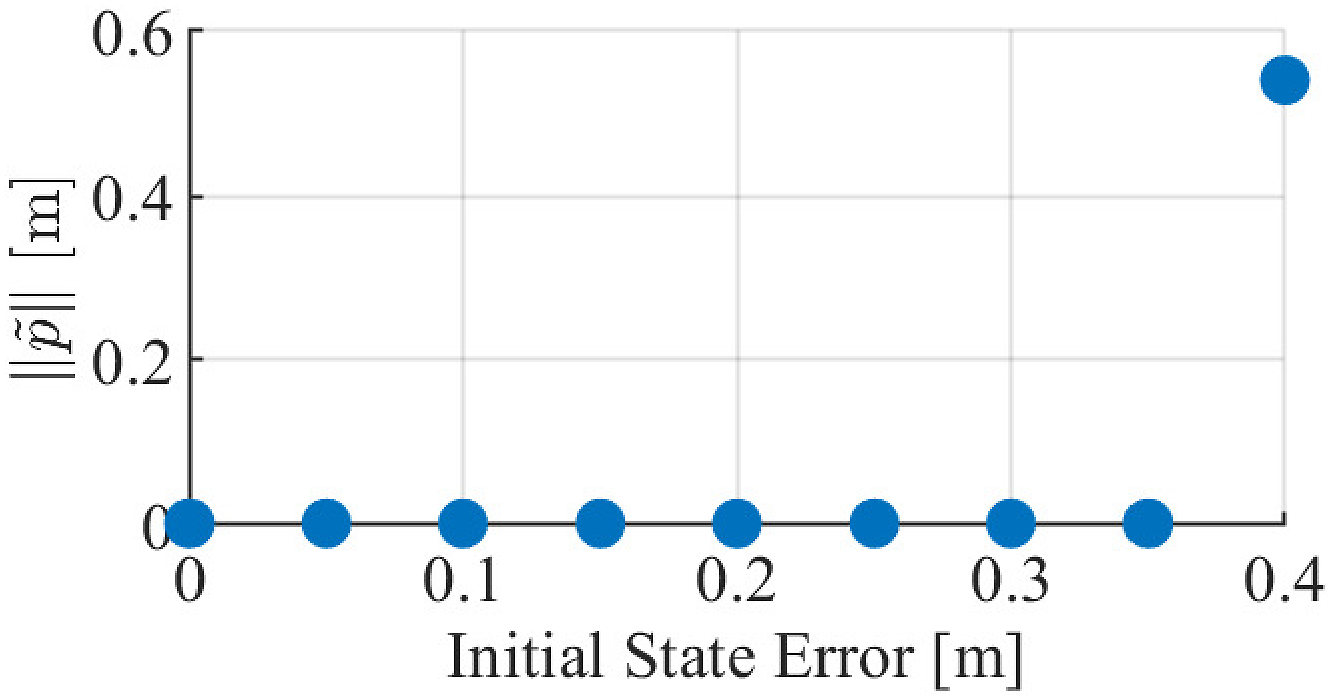

6. Conclusions

In the present work, we introduced a novel approach for the localization of magnetically actuated robots under two EPMs by means of an IMU and magnetic field sensor. We discuss how the relative pose between two EPMs affects the observability of the system and show that alternative EPM configurations ensure localization accuracy without loss of manipulability. Although we have shown the case for two EPMs, the method is easily applicable to additional EPMs, as long as the singularity conditions are studied and defined.

To ensure accurate localization estimates, the platform needs to be calibrated, that is, the relative pose between the EPMs must be known. In this work, we proposed a calibration method that relies on a single triaxial magnetic field sensor and sees the EPM travel an optimized path to ensure the whole workspace of 20 × 20 × 20 cm³ is accurately calibrated.

We tested our localization technique on an SCR and showed that we are able to accurately track the SCR tip 6-DOF pose across the workspace in real-time simultaneously to actuation under 2 EPM control. Overall, the localization achieved errors of 3.5 mm in position norm and 0.21% in orientation, with an error of 2.8° for rotation around gravity during the first 5 min of running. These values are comparable to previous magnetic localization works, such as Taddese et al. (2018) which estimated the full 6-DOF pose under a single EPM system (with average errors of 5 mm), and Fischer et al. (2022a) which only estimated the 3D position under a multi-coil system (with average errors of 2.74 mm). In addition, by evaluating the performance of the algorithm in open space, the SCR experienced higher deflections and faster state-transitions than would be expected in a clinical scenario. As this real-time localization approach is used in future navigation scenarios where these transitions are less pronounced we do not expect a drop in performance.

The orientation was estimated independently from the position by applying a common observer in the special orthogonal group to the accelerometer and gyroscope measurements. This brings the advantage having an orientation estimate that is unaffected by EPM movements and magnetic field measurements. However, it requires accurate initialization and it drifts over time due to the gyroscope bias. Since the estimation of the position relies on the orientation being known, orientation errors will eventually affect the estimation of the position. A solution is to initialize and reset the orientation estimate every few minutes by applying a static localization method (da Veiga et al., 2023).

Additionally, in this work we showed that singularity regions can be avoided without losing manipulability of the SCR. Future work will see the full development of an EPM path planning solution to ensure continuous and autonomous SCR actuation while maintaining localization observability, by avoiding the singularity conditions here defined. In addition to the localization method described here, this will require an accurate model of the SCR to correctly predict its actuation given the EPMs poses. Furthermore, such a model would also contain information regarding the internal magnetic field and how it changes with SCR deflections. This model could also be added to the current localization algorithm aiding with the elimination of orientation drift and position estimation.

The refresh rate of the proposed algorithm was 280 Hz, thus enabling closed-loop control strategies ( $>100$  Hz). This rate is highly dependent on the state estimator used. In this work, an EKF was used as it has been demonstrated to be accurate and reliable for localization strategies. However, more computationally expensive algorithms, such as Particle filters, might provide better estimates at the cost of a reduced refresh rate. On the contrary, simpler methods such as complementary filters might enable much faster refresh rates but less reliable results. Ultimately, the choice of estimator will depend on the specific application and risk susceptibility.

Lastly, the current SCR diameter of 6 mm is limited by the size of the embedded sensors. While this is compatible with applications with larger operating channels, such as gastroscopy (Lloyd et al., 2021), further advances in the manufacture of the such sensors (Xu et al., 2022a) will allow its further miniaturization and application in other areas such as bronchoscopy and endovascular where tools with smaller diameters are needed.

Supplemental Material

Supplemental Material