
Abstract
This paper discusses the design and development of a new Modular, Autonomously Reconfigurable Serial manipulator platform for advanced manufacturing, termed as the MARS manipulator. The platform consists of i) an 18-Degree-of-Freedom (DOF) serial-link manipulator capable of locking any of its joints at any position in their continuous range, such that it can emulate fewer-DOF serial manipulators with different kinematic and dynamic parameters, and ii) an integrated simulation and design environment that provides control over the manipulator hardware as well as a toolset for the design, implementation and optimization of a desired manipulator configuration for a given task. The effectiveness of the MARS manipulator to adapt its configuration to various tasks is examined by assuming two well-known configurations, SCARA and articulated, and by performing a specific task with each of them. The variation in effectiveness of the two configurations in terms of the end-effector trajectory, end-effector accuracy and power consumption is discussed. Further, these configurations are optimized with respect to their performance accuracy, and compared to their pre-optimized versions. Finally, the accuracy model of the simulation is compared against the physical hardware system, running the same task.
Keywords
Introduction
The field of advanced manufacturing constantly strives for the ability to produce a wider range of customized products within a single manufacturing system. Such a need is driving technology towards more adaptive and flexible manufacturing machines, capable of changing their abilities to suit the given task. This mass customization of manufacturing is currently of great interest to both academia and industry [1, 2, 3].
Before the invention of robotic manipulators, manufacturing facilities were dominated by fixed, single-purpose manufacturing machines. Such machines would repeat the same task over again, with little or no variation. Robotic serial manipulators were introduced to be adaptable to a wide range of tasks. Through software re-programming and minor hardware modification, such as changing the end-effector tool, the same robotic hardware is capable of performing a range of fundamentally different tasks, such as welding, riveting, pick-and-place operations, soldering, painting, etc.
Despite their adaptability for various applications, different classes of serial manipulators have emerged that are better suited for particular tasks. The five main classes of serial manipulators are Cartesian, cylindrical, spherical, Selective Compliance Assembly Robot Arm (SCARA), and articulated [4]. Each of these groups of manipulators can range from four to six Degrees of Freedom (DOFs), depending on the wrist configuration mounted on the arm. While there is significant overlap in the task capabilities of these five categories, they have specific advantages and disadvantages for various tasks.
Reconfigurable robotic serial manipulators are a class of serial-link manipulators that are able to emulate a range of serial configurations. By including or removing joints, changing their relative positioning and adjusting the control gains and software accordingly, a reconfigurable serial manipulator can alter its kinematic, dynamic and control properties to suit a much wider range of tasks than that of their conventional counterparts. This field has been researched only sparsely for the past 20 years. One of the earliest works was a pneumatically-powered manipulator called the Reconfigurable Modular Manipulator System (RMMS), which consisted of revolute joint modules [5, 6]. More recent systems include a robot with revolute and prismatic modules [7, 8], and a system with multi-DOF modules [9]. An early attempt at an autonomously reconfigurable serial manipulator is presented in [10]. Its major shortcomings are its limited potential DOFs due to a lack of strength in joints closer to the base. The authors propose to remedy this problem by implementing cascading module sizes allowing for more powerful and heavier modules near the base, and lighter modules near the end-effector, in a similar manner to the manipulator proposed in this paper. In addition, several reconfigurable parallel manipulators have been reported in the literature. These parallel manipulators have different task-properties than their serial counterparts, yet share the same principles of reconfigurability. A three-DOF reconfigurable parallel manipulator is presented in [11], in which an additional actuator changes the kinematics and dynamics of the manipulator, allowing for continuous and automatic reconfiguration of elements of the manipulator. A parallel manipulator named “Cheope” [12] is capable of altering its DOFs by transitioning into eight discrete configurations. Another parallel manipulator, named ReSl-Bot [13], is a fixed six-DOF robot, which uses an additional three DOFs to automatically alter the manipulator's kinematics and dynamics continuously. A common design criterion in all of these works is the ability to change their effective number of DOFs. Both the serial and parallel manipulators accomplish this by either manually re-assembling manipulator modules or re-orienting existing modules through additional module actuators. The former strategy allows for drastic changes between discrete configurations, while the latter allows for smaller changes across a continuous range of configurations, at the cost of added complexity and weight.
This paper presents a new modular, autonomously reconfigurable serial (MARS) manipulator which is capable of autonomously changing its hardware and software to emulate a continuous range of serial manipulator configurations. Its main advantage over its predecessors is its ability to reconfigure autonomously to arrive at a virtually infinite range of configurations. Section II presents the design concept and hardware and software of the MARS manipulator. Section III presents an experimental validation of the manipulator in which it emulates two existing manipulators and each configuration is adjusted based on the performed task. Section IV discusses the results of the experiment, and some concluding remarks are made in Section V.
The MARS Manipulator CAD and Physical
Concept
From a structural standpoint, a reconfigurable manipulator can be thought of as a redundant manipulator with an excess of DOFs required to perform a specified task, and as such capable of performing such tasks with a subset of its DOFs. However, from a performance standpoint the difference between reconfigurable and redundant manipulators lies in how the robots utilize their extraneous DOFs when performing a task. Redundant manipulators utilize their extra DOFs during runtime to satisfy additional task requirements. These requirements can include optimizing one or more criteria, such as energy consumption or accuracy, or additional activities, such as obstacle avoidance. Reconfigurable manipulators, on the other hand, use a subset of their DOFs during task runtime.
This subset is selected offline in order to optimize the same criteria as in the redundant case. While a redundant system may have a better performance for a given task, it may not necessarily be optimally efficient in terms of system complexity (with respect to both structure and control) and energy consumption, since all joints are assumed to remain active during the operation. Meanwhile for a reconfigurable manipulator the system can be configured to use a minimum required number of DOFs with suitable joint parameters to end up with a simpler and more energy-efficient system for performing a given task.

Layout of Module A (smallest module)
The MARS manipulator platform is made up of two major components: a reconfigurable serial manipulator (henceforth referred to as the manipulator), and an Integrated Design and Simulation Environment (IDSE), which allows the end-user to select or design the manipulator configurations, simulate the operation in a virtual reality environment, and operate the physical manipulator and access real-time feedback and recorded data; this is discussed in detail later in this section.
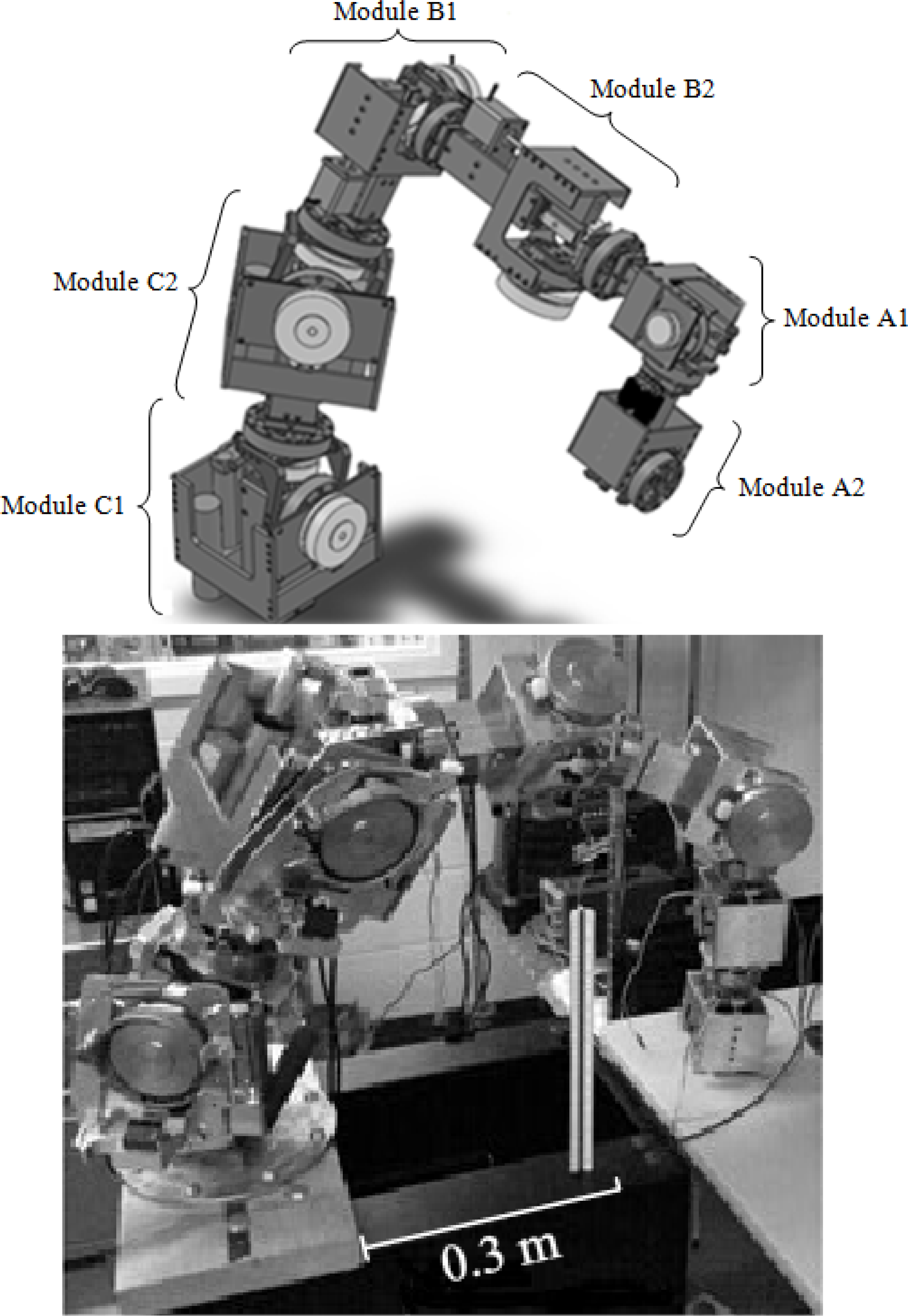
The manipulator hardware and its CAD model are shown in Figure 1. The manipulator has 18 DOFs, consisting of 12 revolute and six prismatic joints. It is able to physically reconfigure itself with fewer DOFs either to emulate existing serial manipulator configurations or to create new configurations. The reconfiguration is achieved through utilizing the 18 DOFs and then locking specific joints, so that with the resulting unlocked joints a desirable kinematic configuration can be achieved. Once the configuration is set, only the unlocked joints will be actuated.

Module Link Diagram
The joints are grouped into six modules, each with three joints, as shown in Figure 2. Each of the modules has the same geometric layout, consisting of one prismatic joint and two revolute joints, which are mutually perpendicular (P⊥R⊥R). Each module is connected to the previous one so that the kinematic layout for the complete manipulator is (P⊥R⊥R||P⊥R⊥R|| … ||P⊥R⊥P). This layout was selected for three reasons. First, many serial manipulators have a wrist mechanism located at the end of the manipulator. The wrist configuration is usually either roll-pitch-roll or only pitch-roll. Such a wrist configuration would be readily available with the selected layout, aiding in creating existing configurations, as well as in developing new configurations effectively. Further, having such a wrist in each module, located throughout the manipulator, increases the versatility of the reconfiguration task. The second reason for the selected manipulator layout is that by having the first DOF in the module as a prismatic joint, various link lengths of the final configuration can be achieved. Without a prismatic motion capability, link lengths would be limited to combinations of unchanging module lengths, which would drastically reduce the variety of the possible configurations that the manipulator can assume. The third reason for the selected manipulator layout is related to the mutual orientation of the three DOFs of each module, as well as the orientation of the adjacent modules. With their selected layout orientation, it is easy to have two or more prismatic joints parallel to each other. This allows for the stroke of the prismatic actuators to stack, increasing the stroke of the active DOF. The stacking of actuators also allows a significant increase of the speed of linear actuation, which is a design issue for serial manipulators employing a prismatic DOF.
The following assumptions were made about the modules: i) the centre of mass of each module is located at a distance l1 from the base, coincident with joint 2; ii) the masses of the partial module before and after joint 2 are equal. Both of these assumptions eventually become trivial when the worst-case scenario is assumed for equations (12) and (13).
The design of the manipulator modules was subjected to optimization. First, the Jacobian for a generic module was developed. Each module can be treated as a three-DOF serial manipulator. The module's Jacobian (MJ), expressed in the module frame {M} is defined as:

where
Given the link diagram in Figure 3, the module's Jacobian expressed in frame {M} is:
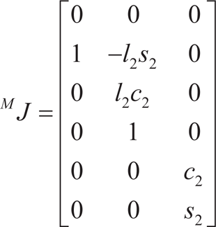
where c2: = cosq2 and s2: = sinq2
The expression of the Jacobian in frame {E} can be obtained using the rotation matrix between frames {M} and {E}:

The force/torque matrix

A basic functionality requirement for the MARS manipulator is to lift a 1 kg mass 10 cm beyond the last module, representing the end-effector. To ensure that the manipulator can handle such a payload at any orientation, the maximum applied wrench to the sixth module is assumed as:
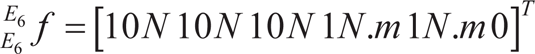
The moment component in the z-direction was omitted as it does not affect module 6. For simplicity, the pre-superscript and pre-subscript for an applied wrench are omitted as follows:

Given the manner in which the modules are connected, the frame {Mi} is the same as frame {Ei−1}. The applied wrench to the subsequent modules can, therefore, be given by the following recursive equation:

where

and


From equations (4) and (7), the joint torque for each module can be calculated due to an applied static wrench. In addition to this load, each module must be able to lift the weight of the modules after it. To calculate this additional load, assume that the centre of mass for each part of a module is located at its midpoint. Then, the y-component of the centre of mass for module j in {M} is:
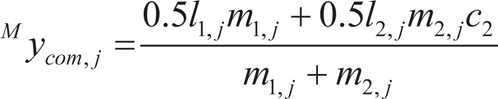
Assuming that the mass of the two parts of each are equal and considering a worst-case scenario where all modules after a module a have q2 = 0, the distance of the centre of mass of module b from the end of module a can be as follows:
In this case, the equivalent wrench applied to the end of module a due to the force of gravity of module b is described as:

The expression of vector
To include the gravitational wrench, equation (7) can be amended as follows:

where

The above equations describe the wrench applied to all modules due to a static load and the forces of gravity. Through utilizing equation 4, this can be transformed into joint force/torque. Although a worst-case scenario is considered for the effect of the gravitational wrench in equation (14), the expressions MyE and MzE must still be assumed for configurations which create maximum joint force/torque. The first part of equation (14) must also be computed for maximum joint force/torque. However, the identification of such configurations is computationally prohibitive for a design optimization task.
To simplify the problem, equation (14) can be modified to apply gravitational forces and moments to joints directly. Due to a feature of the manipulator's geometry, joint 2 of module j must take the moment due to the gravity from all modules from j+1 to 6, whereas joint 3 must take the moment due to the gravity from modules j+2 to 6. Therefore, the maximum joint torque for each module in response to the applied load and the weight of each module can be simplified to:

where fj can be computed from equation (7).
The second simplification is applied to the matrix

Intuitively, this matrix makes sense, as the force applied to each module will be the same (10 N in each principle direction), and the moment will be the original moment (in the xM and yM directions, corresponding to joints 2 and 3, respectively) plus the added moment of the applied force at an offset.
To find the maximum force/torque for each joint, equation (17) is resolved for q 2=−90o, −45o, 0o, +45o, +90o. The value of q 3 does not affect this torque, and the value of q 1 is set at its maximum stroke of 50 mm.
To optimize the design parameters of all six modules of the MARS manipulator, the following cost function was considered:

where

subject to
where


Length 1 Optimized and Actual Values

Length 2 Optimized and Actual Values

Module Mass Optimized and Actual Values
The first constraint assumes that in every module l1 is twice that of l2. This constraint is made to accommodate the additional actuator that the first half of the module must contain. The second constraint assumes an overall length of the manipulator in order to provide a suitable workspace. The manipulator is a table-top robot, with a desired reachable workspace of 2 m3. The structural length index of the robot, given in equation (20), is a measure of how efficiently a robot utilizes its size to create a workspace [14].

where L is the length sum of the manipulator as the sum of the links’ lengths and offsets, and W is the volume of the reachable workspace. Traditionally, a QL value of between 1 and 1.3 is considered desirable for an articulated serial manipulator containing a combination of prismatic and revolute joints [15]. Hence, choosing a conservative index of 1.3 for QL with the desired workspace gives a length sum of 1.64 m.

Joint Force Optimized and Actual Values.
The third and fourth constraints enforce the types of modules. The six modules would be grouped into types A, B and C, as shown previously in Figure 1. This reduces the design and fabrication time of the manipulator as well as the cost, as only three types of module are to be produced, instead of six.
The fifth constraint ensures that the resulting masses of the modules are sufficient to provide the required torque. Three factors are used: a structure factor (SF), a prismatic actuator factor (A), and a revolute actuator factor (B), defined as SF = 1.5, A = 25 N/kg and B = 300 Nm/kg. The actuator parameters were obtained by comparing a variety of available brushless DC motor and gearbox combinations, specifically the EC-flat line of Maxon motors with SHD harmonic drives and the Firgelli linear actuators. It was found that most of these actuator systems have force/torque-to-mass ratios close to these factors. This is only an approximation, but it serves to constrain the optimization into realistic module masses.
Prismatic Joints.
Revolute Joints

Figures 4 to 6 show the results of the optimization for the module lengths and masses, as well as the actual lengths and masses of the constructed MARS manipulator. The constructed manipulator was not able to exactly follow the guidelines that were resulted from the optimization, due to the discrete selection of the off-the-shelf components. The mass of the MARS manipulator was reduced where possible, as a larger mass is never advantageous. The optimization simply gave an upper bound for the mass.
From the optimization, the resulting maximum values of joint force/torque were calculated using equation 17. These values are compared with the actual actuator values used in the MARS manipulator in Figure 7. Note that the optimized value for the linear actuators (joints 1, 4, 7, 10, 13 and 16) are significantly higher than the optimized value. This was a design decision based on the fact that a linear actuator must always move the maximum mass of the manipulator, while revolute actuators move a varying, and often decreased, effect of moment of inertia. The only actuators below the optimized worst case were joints 3 (slightly), 9 and 15. All of these are the roll actuators in their respective modules. A more powerful actuator in these modules would have violated the mass requirements. Instead, the length of modules B and C and the mass of module B were reduced below the optimized value, reducing the demand on these actuators. It is still worth nothing that these joints represent the weak point of the manipulator.
Tables 1 and 2 show the actuators specified for each module. Linear speed near the base and end of the manipulator was compromised in favour of weight and size, as it is uncommon for useful configurations to need high-speed linear joints in these locations. Similarly, near the base, speeds for the revolute joints were traded for weight, as lower joint speeds near the base can still produce the same end-effector speeds, due to the longer-moment arm.
Braking Mechanism

MARS Software Architecture
The gear reduction for all revolute joints was accomplished they are very compact, which was necessary for satisfying through harmonic drive systems. These gearboxes were the lengths reported from the optimization; and thirdly, chosen for three reasons: first, they have zero backlash, they have integrated cross-roller bearings to protect the which is an important feature in robotic joints; secondly, gearboxes and actuators.
MARS IDSE Interface
Each joint has position feedback through Hall-effect sensors, potentiometers and encoders. Force feedback is accomplished by a cantilever beam in each module which bears 100% of the linear force. A strain gauge on these beams can measure the amount of deflection and translate it accurately into the force experienced by the linear actuator. A similar technique is employed for the torque in the rotary actuators. A cross composed of four beams is attached to the output of each revolute joint. By applying strain gauges to each of the four beams, the force in each beam can be measured, translating into the torque.
In order for the manipulator to reconfigure itself to resemble fewer-DOF manipulators, it needs to effectively remove selected joints from its kinematic layout. The joints, however, must be removable in a continuous range of positions. Non-backdriving locking brakes were designed for each joint, which can be engaged in any of the motor positions, as shown in Figure 8. Consequently, each DOF has the capability of holding its position statically with any continuous displacement.

Articulated Simulated Manipulator

SCARA Simulated Manipulator
The software platform for the MARS manipulator is separated onto two PCs, as shown in Figure 9. The first one, called the target machine, acts as a real-time kernel for operating the manipulator. The second PC, called the host machine, runs the design and simulation modules, and controls the real-time operation of the target machine. The host machine is accessible by remote users through the Internet, as well as locally.
Workspace vs. Link Length
Workspace vs. Link Length

Position and Time Checkpoints for the Task

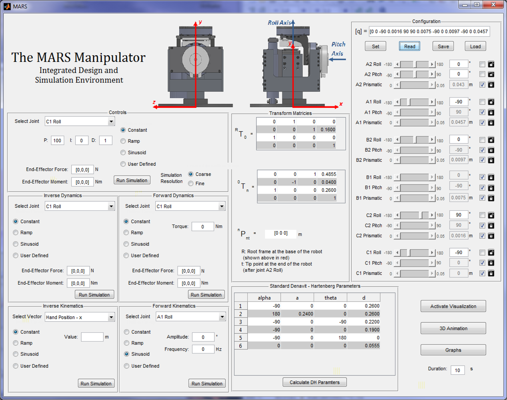
The host machine runs an Integrated Design and Simulation Environment (IDSE), where users can design a suitable configuration and control parameters for the MARS manipulator for a given task, simulate its performance, and load the configuration onto the physical setup. The host software is based on the MVC (Model-View-Controller) architecture [16, 17], and is developed within the MATLAB/Simulink® environment, utilizing SimMechanics™ physical modelling and animation modules. The IDSE is capable of performing five types of simulation: inverse kinematics, forward kinematics, inverse dynamics, forward dynamics, and controls. It also provides kinematic information on the current configuration in the form of a DH (Denivit and Hartenberg) table and transformation matrices. The visualization engine provides a 3D model of the current configuration, as well as a 3D animation of the most-recently-run simulation. There are also built-in data acquisition functions to record joint kinematics and dynamics and end-effector motion. Further, the IDSE works with the Simulink® design optimization and MATLAB® optimization toolboxes to optimize the configuration based on a user-defined task. The IDSE's graphical user interface is shown in Figure 10.
To demonstrate that the MARS manipulator can effectively be reconfigured to various configurations with their associated advantages, an experiment was performed involving two common configurations. The two arm configurations selected for the experiment were the articulated configuration (R⊥R || R) and the SCARA configuration (R || R || P), and they were first simulated in the IDSE (Figures 11 and 12).
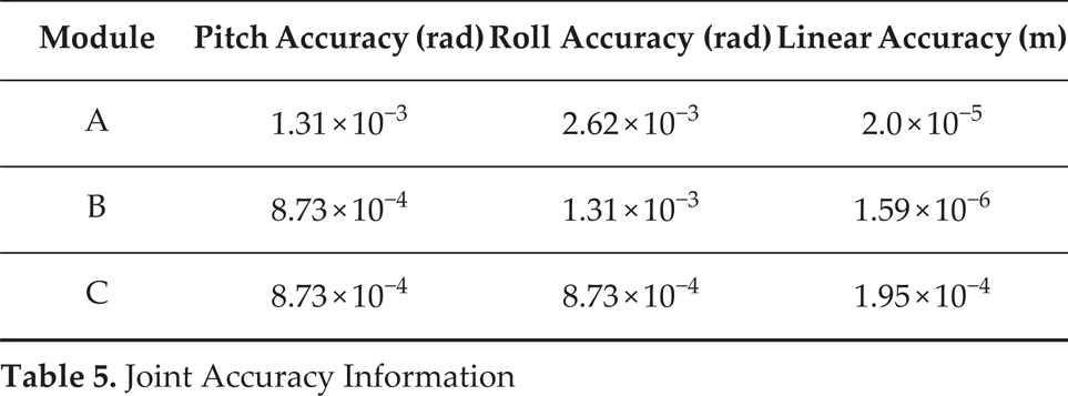
Joint Accuracy Information
Joint Accuracy Information
The articulated and SCARA configurations have known advantages and disadvantages associated with their practical application. The most prevalent advantage of an articulated serial manipulator is its high workspace volume for a given amount of material in the arm structure (indicated by the arm's length sum), which is measured by the structural length index QL, given in equation (20). Table 3 illustrates this ratio for the two configurations of the MARS manipulator.

Articulated End-Effector Trajectory
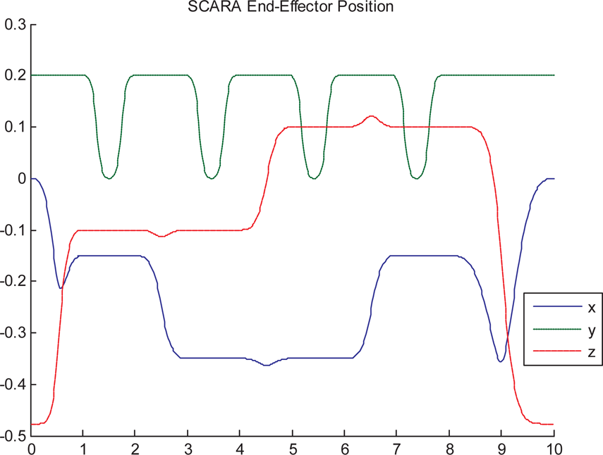
SCARA End-Effector Trajectory
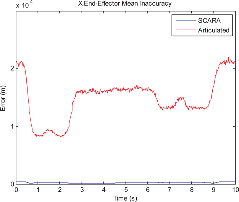
X End-Effector Mean Error

X End-Effector Error Standard Deviation
The smaller QL for the articulated configuration translates into a greater range of tasks this manipulator is capable of undertaking.

Y End-Effector Mean Error
The advantage of a SCARA configuration over the articulated counterpart is its greater accuracy in the planar positioning of its end-effector. To illustrate this, an experiment imitating a spot-welding operation was performed for each manipulator configuration, first in a simulation environment and then with the physical robotic hardware. Four target points were labelled (P1 through P4) on a plane in the manipulator workspace. The manipulator approached 20 cm above each target point, then lowered and raised the end-effector to touch the point, keeping its x and z coordinates constant. This process was repeated for all target points. For the entire task, the approach vector remained in the −yR direction. Table 4 lists a time sequence for the task.
Configuration comparison
Three characteristics associated with the defined task are discussed in this section: the end-effector positioning end-effector accuracy, and total manipulator power consumption.
The end-effector trajectories for the two manipulator configurations are shown in Figures 13-14. The x, y, and z components refer to the end-effector point coordinates in frame {R} (Figures 11-12). From these graphs, a few interesting characteristics of the configurations are revealed in terms of manipulator simplicity. Recall the conditions of the task, where the end-effector needed to move linearly only during the approach in the −y direction, henceforth referred to as the approach segment. For these time periods [1:2], [3:4], [5:6] and [7:8] the x and z values are constant for both configurations. The SCARA configuration accomplished this criterion by performing inverse kinematics at eight points in the workspace: at each of the target points P1 - P4 and at 20 cm above each of these four target points. Then, the manipulator was instructed to move between the points, as moving linearly is a feature of the configuration. For the articulated configuration, inverse kinematics (which was modified from the closed-form inverse kinematics of the PUMA manipulator in [18]) was performed for the same eight points, as well as for an additional 160 points during the approach segment. Note that for the time periods [2:3] and [6:7] where the additional points were not computed, the SCARA configuration has a constant y value, whereas the articulated configuration has a non-constant y. Further, the inverse kinematics equations for the SCARA configuration consist of 50% less code when compared to the articulated configuration, further decreasing the runtime as well as the time to set up the task on the part of the programmer.

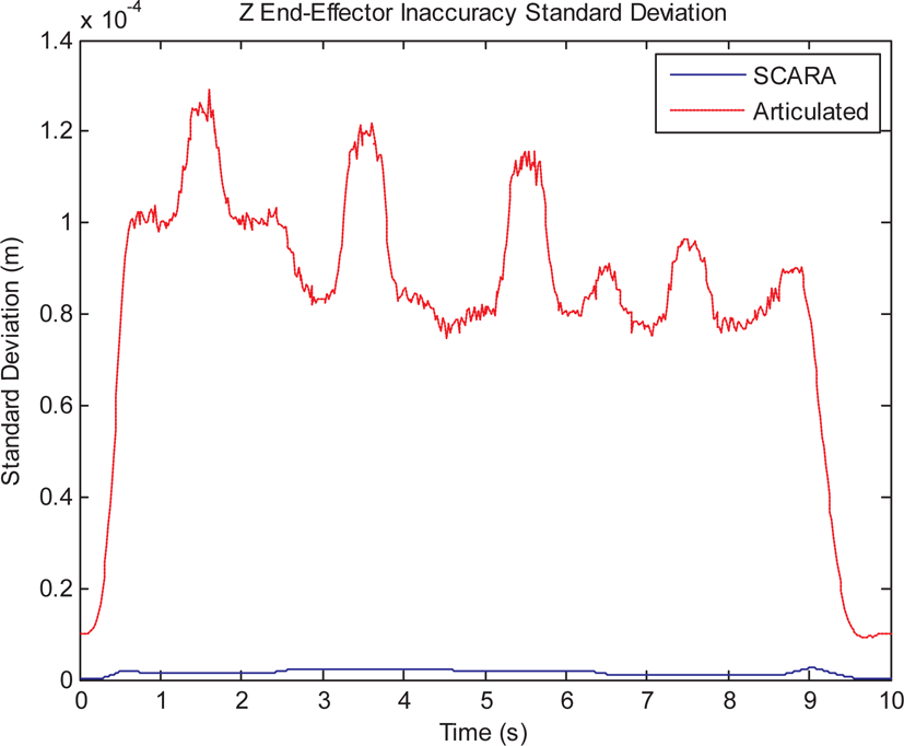
Z End-Effector Error Standard Deviation

Z End-Effector Mean Error
The end-effector accuracy is calculated from the sensor accuracy for each joint. There are four variables that describe the relevant accuracy for this task: Δx, Δy, Δz and Δθ. The first three of these variables give the translational error of the end-effector in the three principle directions: x, y, and z. The fourth variable, Δθ, describes the error in the approach vector of the end-effector. The orientation vector and the normal vector are ignored as they are not of concern for a spot-welding task.
To obtain the accuracy metrics, first the forward kinematics of the manipulator is observed at the ideal joint positions. This obtains the following end-effector position and approach vector:
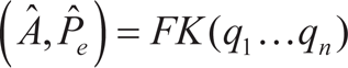
where qi is the displacement of the ith joint and n is the number of DOFs of the manipulator's configuration.
Y End-Effector Error Standard Deviation
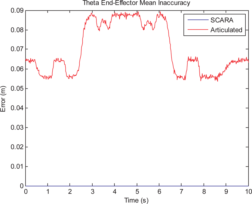
Theta End-Effector Mean Error
The forward kinematics is observed again, this time with a perturbation of the joint position based on the accuracy of the joint:

where r is a random number in the interval [−1,1] and i is the accuracy of joint i, defined in Table 5.
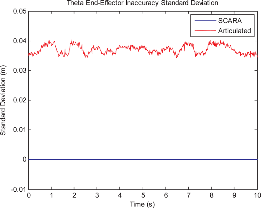
Theta End-Effector Error Standard Deviation

Task Power Consumption
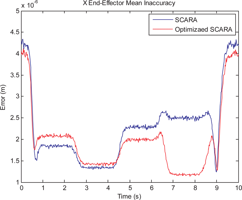
X End-Effector Error Optimization for SCARA

Z End-Effector Error Optimization for SCARA

X End-Effector Error Optimization for Articulated
The translational error is calculated as follows:

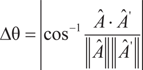
The error in approach vector is calculated as follows:
The random number r is part of a Monte Carlo statistical accuracy model similar to those used in [19] and [20]. Without this term, equations (23) and (24) would provide the maximum possible end-effector error. To compute for the Monte Carlo model, the accuracy was calculated for each joint 2,000 times, and the resulting mean and maximum values were obtained. Figures 15 to 22 show the resulting mean and standard deviation of the end-effector errors for each of the four accuracy metrics. From these graphs, it is clear that the SCARA configuration has superior accuracy compared to the articulated configuration. The only exception is in the y direction. This is due to the fact that in the SCARA configuration motion in the y direction is controlled by four separate linear actuators working in parallel, which increases the overall error. However, this error is still comparable to the error from the articulated configuration for this direction. For the error in approach vector (Δθ), it is a feature of the SCARA configuration that this error remains zero for any position of the end-effector.

Y End-Effector Error Optimization for Articulated

Z End-Effector Error Optimization for Articulated
A final characteristic of the task that was analysed was the manipulator power consumption, shown in Figure 23. For motion between points, the SCARA configuration used approximately half of the power needed for the articulated configuration. For the approach segment, the SCARA configuration used between two and six times as much power as the articulated configuration. This is due to the linear motion for the SCARA configuration being produced by four separate linear actuators working in parallel, as mentioned previously for the accuracy model. In total, the SCARA configuration used twice as much power on average compared to the articulated configuration. The above results highlight the advantages and disadvantages of the articulated and SCARA configurations when assumed by the MARS manipulator platform.

Theta End-Effector Error Optimization for Articulated

Objective Function for SCARA

Objective Function for Articulated
Waypoint Accuracy for Simulated Data

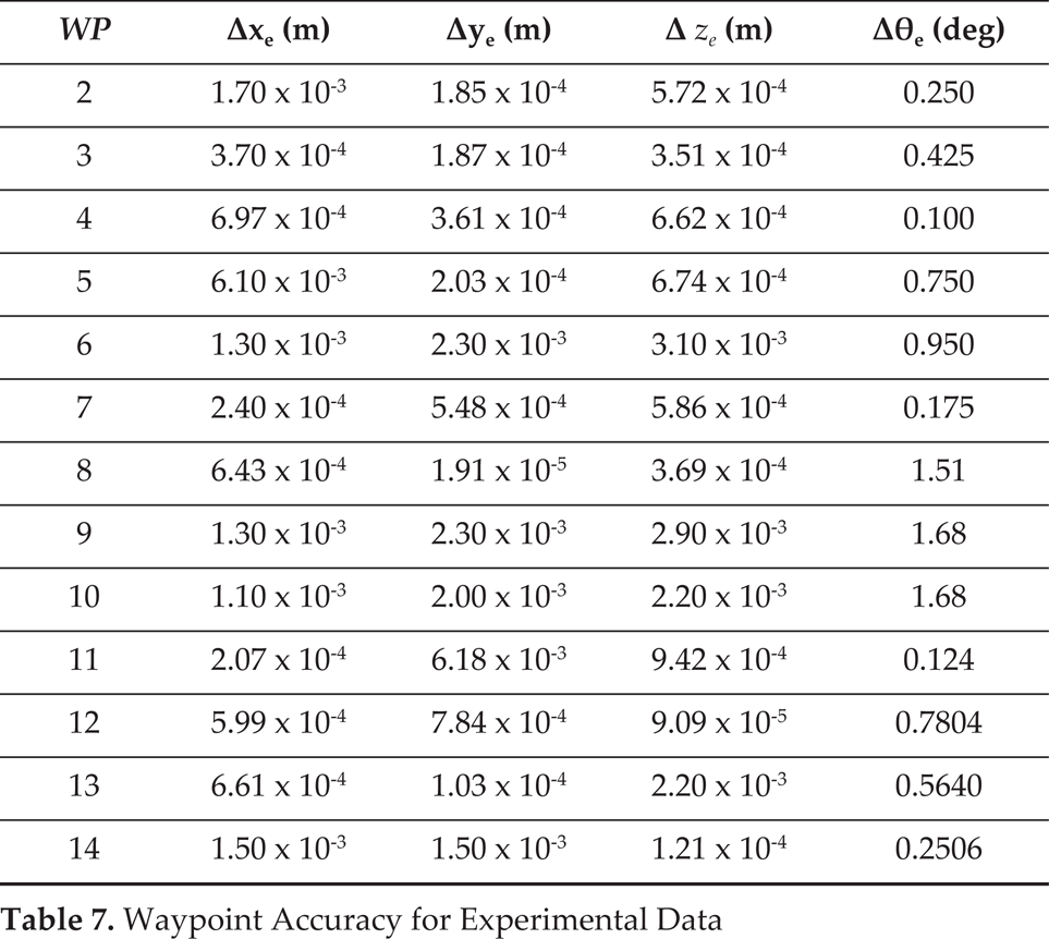
Waypoint Accuracy for Experimental Data
In the previous section, the differences in the performance of the MARS manipulator were explored for the two configurations. These configurations, however, represented just one of infinitely many versions of the SCARA and articulated class manipulators that the MARS manipulator can assume. Within a specified class of manipulator, the link parameters can be optimized against a variety of criteria. In this section, each of the two configurations previously discussed are optimized against the accuracy criterion. The objective function for this optimization is given as:

subject to

where li is the ith link length that the MARS manipulator is capable of varying, and l and ϕ are characteristic lengths and rotations used to normalize the errors. The values for l and f were taken as 1 mm and 1°, respectively. Using the MATLAB/Simulink® optimization toolboxes, the configurations were optimized based on the objective function, and the task was performed again for each configuration. The resulting manipulator accuracies are shown in Figures 24 to 29, and the value of the objective function in equation (25) is shown in Figures 30 and 31. Note that link lengths only affect the x and z accuracy for the SCARA-class manipulator, while x, y, z and θ accuracies are affected for the articulated class.

Joint 1 Experimental vs. Simulation Trajectory

Joint 2 Experimental vs. Simulation Trajectory
It was shown in the previous section that the MARS manipulator was capable of inheriting the advantages of both the SCARA and articulated configurations. This section shows that, through an optimization, both configurations can be improved through varying their link-lengths. These two actions, choosing a configuration class and optimizing the link-lengths, can be thought of as coarse and fine tuning of the manipulator configuration.

Joint 3 Experimental vs Simulation Trajectory
To help validate the simulation model, the spot-welding task was repeated on the physical MARS manipulator hardware in the articulated configuration. The joint trajectories for the articulated arm (joints 1-3) are shown in Figures 32 to 34.
The experimental data were processed through a noise-reduction filter, as the sensor data had periodic outlier errors. Note that, for the experimental data, the speed of the task was reduced, so as to prevent damage to the hardware manipulator. As such, the 14 waypoints are highlighted on the graph to compare with the simulation results. The difference between the simulation results and the experimental data is largely due to the task implementation. The simulated results perfectly follow a cubic position profile, keeping acceleration from becoming unreasonable. For the experimental results, a PID controller was used to transition between waypoints, causing the motion profile to be determined by the controller.
The accuracy of the experimental hardware was also compared to the accuracy of the simulation. The two accuracies are shown in Tables 6 and 7. From these tables, it is clear that for most instances, the accuracy of the experimental results is comparable to the accuracy of the simulated data. There are some exceptions, most notably at waypoints 9 and 10. However, for waypoint 8, the position accuracy of the experimental data is very close to the simulated data. Given that waypoints 8 and 10 are the same point in both joint and end-effector space, this means that the inaccuracy is not position-dependent, but is rather likely to be due to the above-mentioned sensor noise. Another potential source of such an error could be the manner in which the end-effector approached the way-points. Waypoint 8 was approached through a planar arc, while waypoint 10 was approached from a linear vertical motion. This is unlikely to be the case in here, as waypoints 5 and 7 shared the same property as waypoints 8 and 10. However, in the first case, waypoint 5, which was approached by a planar arc, experienced the higher error value. In the second case, waypoint 10, approached by a vertical linear motion, experienced the higher error value. Ignoring these outlier cases, the experimental data and the simulated data for accuracy are quite similar, validating the accuracy model used in the previous optimizations.
Conclusions
In advanced manufacturing and mass customization, having a tool available which can adapt itself for a wide range of tasks is essential. The design and development of a robot manipulator platform was discussed in this paper that is capable of emulating a continuous range of existing and new manipulators. It was shown that by varying the parameters of the manipulator, it was able to expand its workspace, increase its accuracy, or improve its power consumption. Further, once a class of configuration is chosen, the configuration can be optimized against any set of specified criteria to further improve performance.
Future work for this manipulator system will investigate the potential for optimizing configuration class based on a given task. Specifically, we will explore configurations where joints are neither perpendicular nor parallel to their surrounding joints. This would allow the manipulator to explore new types of configurations that would only be useful for a narrow range of tasks, which have therefore previously been unfeasible for fixed-configuration manipulators.
Acknowledgements
This work was financially supported by MathWorks®, Inc., through the Curriculum Development Fund.