Sage Journals: Discover world-class research

Abstract

This research presents two novel approaches to nonholonomic motion planning. The methodologies presented are based on the standard fast marching square path planning method and its application to car-like robots. Under the first method, the environment is considered as a three-dimensional C-space, with the first two dimensions given by the position of the robot and the third dimension by its orientation. This means that we operate over the configuration space instead of the bi-dimensional environment map. Moreover, the trajectory is computed along the C-space taking into account the dimensions of the vehicle, and thus guaranteeing the absence of collisions. The second method uses the standard fast marching square, and takes advantage of the vector field of the velocities computed during the first step of the method in order to adapt the motion plan to the control inputs that a car-like robot is able to execute. Both methods ensure the smoothness and safety of the calculated paths in addition to providing the control actions to perform the trajectory.

Keywords

Nonholonomic Path Planning Fast Marching Square

1. Introduction

Path planning and the control of autonomous vehicles has become widespread, not only in industry but also in everyday life. Currently, several cars in the market offer autonomous parking systems, there are robotic vacuum cleaners in millions of houses around the world, and the use of unmanned aerial vehicles is increasing every day in many different application fields. All these applications require the vehicles in question to be capable of working in a robust manner under a wide variety of environmental conditions [1], operating without human intervention [2], and providing some guarantee of task performance [3]. For all these reasons, these robots need to be able to plan smooth, reliable and safe trajectories as quickly as possible.

A navigation task for an autonomous mobile robot consists of finding a control strategy so that the robot reaches a desired pose while at the same time avoiding colliding with obstacles in the environment [4, 5]. During the planning step, there are two main research directions that are emerging from the different kinds of robots being used. Some applications focus on robots with simple dynamics and of negligible size, such that it is valid to reduce the problem to a classical navigation task. Different approaches aim to solve the classical navigation problem for mobile robots with complicated dynamics, such as nonholonomic or underactuated systems [6, 7].

The path planning problem is formulated in the configuration space (C-space) [8]. The C-space is the space of all possible states of the robot. Thus, if we consider a rigid robot moving in a two-dimensional environment, the configuration q=[x,y,θ]^T describes the position of the robot in the plane and its orientation with respect to the vertical axis. The majority of planning methods deal with driftless control affine systems, which have the form:

\dot{x} = \sum_{i = 1}^{m} h_{i} (x) u_{i}

(1)

where the state ẋ ∈ X consists of the configuration variables and their derivatives, h_i is a vector field on the state space of X, and u=[u₁…u_m]^T ∈ U is the vector of the control variables. If the configuration is treated as the state, then x=q. A nonholonomic vehicle is a system which obeys one or more non-integrable equality constraints above the derivatives of the configuration variables. This means that the velocity vector is locally constrained to certain directions (for instance, a car is not able to move sideways).

An interesting property of nonholonomic systems is that they are underactuated yet remain controllable on the entire state space - this leads to the development of local control methods which determine the control signal u(·) for a given pair of initial and goal configurations (q_i,q_g), which are called ‘steering methods’ [9]. Among these algorithms, some of them are designed to work in special types of nonholonomic systems: nilpotentizable [10], chain-formed [11, 12] and differentially flat systems [13]. One common problem among these methods is that they are mainly designed to work in the absence of obstacles.

A simple approach to solve the path planning problem in uncluttered environments consists of taking into account only the geometric nature of the model. Therefore, a planner can calculate a set of continuous poses inside the free configuration space, connecting given initial and final configurations of the autonomous vehicle. However, if the problem includes both geometric and kinematic constraints, the above approach may not be sufficient to describe a solution path, since in those cases a suitable path planning algorithm has to find a solution, such that it obeys the motion equation of the kinematic robot model and it is also safe with respect to avoiding obstacles.

In [4, 5], it is shown that the existence of an admissible path between two configurations is equivalent to the existence of any collision-free path between the same configurations. This is still an open research topic since, to the best knowledge of the authors, there is no optimal solution available for the synthesis problem. Most algorithms which propose a feasible solution can be divided into two main groups. The first one includes probabilistic sampling-based roadmap methods [14, 15], which involve iteratively sampling the free space and using local steering methods to connect the samples. The second group of techniques use the previously-mentioned idea of the equivalence between the existence of pure geometric and nonholonomic paths. These methods [16, 17] optimize a not necessarily nonholonomic initial path to obtain a final collision-free concatenation of feasible paths. Both the optimization process and the path planning are based on potential fields and therefore have local minima that cannot be avoided with certainty.

Rapidly random trees (RRT) [5] is a well known sampling-based planner, which is widely used in robotics because of its quick response. However, the generated paths are suboptimal and very often require further iterations to be improved. In this work, the nonholonomic RRT variant for car-like robots (RRT-NH) [18] is used to compare the results obtained with our own method.

This paper describes two variations of the standard fast marching square path planning method (FM²) [19] in order to apply them to nonholonomic vehicles. The approaches have been labelled ‘nonholonomic fast marching square’ (FM²-NH). The first of these approaches begins by precomputing all the feasible and collision-free poses of the nonholonomic autonomous vehicle. Next, the FM² and the gradient method are used to compute a smooth and reliable trajectory based on a velocity potential map., The second relies on the vector field of the velocities computed in the first step of the FM². These vectors are used to adapt the path planning to meet the constraints in the movement of a car-like robot. Both approaches calculate smooth and safe paths while also providing a control plan for the robot.

The remainder of this document is organized as follows. Section 2 provides an introduction to the fast marching path planning method and its extension into the fast marching square algorithm; in Section 3, the adaptation to nonholonomic planning is explained. In Section 4, different simulation results show the advantages of the method. Finally, in Section 5, conclusions are drawn.

2. Fundamentals of the Method

This section presents the most important concepts used in this work as well as the basis for the presented path planning approaches.

2.1 Fast Marching and Path Planning

The principle behind the fast marching method (FMM) is the expansion of a wave: in two dimensions, intuitively, the method simulates the spreading of a thick liquid as it is poured into a board, obtaining the time in which the front reaches every point of the grid. Similar formulations have been used in other study areas such as fluids mechanics, molecular dynamics in relation to electrostatics, thermal analysis, and more. Notwithstanding, it is crucial to highlight that the most important and peculiar feature of the method concerns how the wave expansion is calculated in arrival time for every cell in a grid. As a consequence of its particular mathematical formulation, the outputted potential map of the method presents only a global minimum and no local minimum whatsoever. There are many preceding graph search algorithms based on similar approaches, such as Dijkstra and A*, see [20] and [21] respectively; these search methods have been widely used and demonstrated to be efficient. Conversely, they have been proven to be inconsistent in the continuous space [22].

In an homogeneous environment, the FMM generates - at same levels of the wave - front interface points in circular form and centred around the source location. In such a case, all the points in the interface are reached at a given time homogeneously, and the minimal paths between two points in the space are always composed of straight lines.

The methods foundation is the same as the one behind the Fermat principle in optics, which states that a ray of light which goes through a prismatic glass always takes the fastest path between any two points; in other words, it takes the minimum - or optimal path - in time. The interface - or wavefront - can be a flat curve in 2D, a surface in 3D, or even (although it may not be possible to represent it graphically) mathematically generalized to any number of dimensions. Time T is calculated for every point as the wave advances and covers the grid map; the front denominated G advances always moving in the normal direction. The FMM is able to receive even more than one source point as input, and then the wavefront is generated from each source point. The interface origin points are initialized with T =0 and the frozen state, according to the names of the algorithm states. To obtain the geodesic path over a map, the source point must be unique, which stands for an entirely global minimum T=0, implying that the rest of values will always be greater than zero. The speed F is established by the velocity potential map, and may vary from point to point, but it is always positive or equal to zero within obstacles' grid points. The values of the front are described by the Eikonal equation, as given by Sethian [23]:

1 = F (x) | \nabla T (x) |

(2)

where x is a point in space, F (x) is the speed of the wave for that position, and T(x) is the time required by the wave interface to reach x. Accordingly, the velocity is inversely proportional to the gradient magnitude of the arrival time function T(x):

\frac{1}{F} = | \nabla T |

(3)

2.2 Implementation

The solution for the Eikonal equation can be computed iteratively over a grid map, and the pseudo-code algorithm for the method is shown by Algorithm 1. Before going into the details, we will explain the different labels the cells of the grid map can take.

UNKNOWN: cells whose T value is not yet known because the wavefront has not reached them.

FROZEN: cells whose T value is fixed because they have been passed over by the wave.

NARROWBAND: cells that may be part of the wavefront in the next iteration. They already have a T value assigned, but it can change in future iterations of the algorithm.

The algorithm has three stages: initialization, loop and finalization. During initialization, T =0 is set in the cell in which the wave originates and this cell is labelled as ‘frozen’. Afterwards, all its Manhattan neighbours are labelled as ‘narrowband’ and T is computed for each of them.

In each iteration of the loop in Algorithm 1, the Eikonal equation is solved for the Manhattan neighbours (which are not labelled as frozen) of the cell in the narrow band which has a lesser T value, and this cell is then labelled as frozen. The narrow band consists of an ordered list, from the lowest to the highest T value, of its cells. The finalization is reached when all the cells are labelled as frozen. The output is a potential map with an arrival time value T for each cell. If the descent gradient is applied, it leads to the shortest path in time which, in a map with homogeneous velocity, is the same as the shortest path in distance, and it is called the ‘geodesic’. Figure 1 shows an FMM path between two given points.

Figure 1.

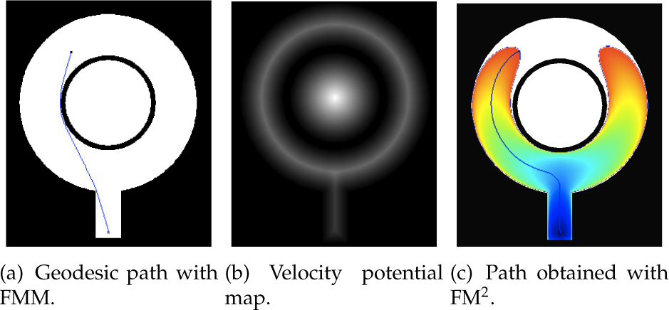
Example of paths obtained with (a) FMM, and with (c) FM². The generation of the (b) velocity potential map.

2.3 Fast Marching Square

The original FMM approach assumes the isotropy of the free space; put another way, the environment map has a uniform velocity value for all the grid positions in which obstacles are not present. It can be seen in Figure 1 that the path obtained using FMM is not safe because it has no clearance from obstacles; nor is it smooth, because it permits abrupt turns along the path. These disadvantages are overcome by the FM 2 method, which we have successfully used with many approaches [24 –27].

The FM² method takes advantage of the ability of the FMM to compute the time arrival values over an anisotropic - or uneven - map. This concept was demonstrated first by Sethian et al. [28]. This means that the velocity in the free space does not need to be homogeneous, and thus a velocity potential map can be defined so that the resulting path overcomes the issues shown by the FMM.

In the case of FM², the velocity potential map is computed using FMM. The result of this step can be seen in Figure 1, in which we can see a greyscale image that takes higher values (white and light grey) the further the positions are from obstacles, and lower ones the closer they are to the obstacles. If we compute the FMM over this map, we obtain a time of arrival map, as can be seen in Figure 1. In this case, the shape of the wavefront is no longer circular, since the velocity is not homogeneous. Instead, the front of the wave for a certain T value (which consists of those positions that have the same colour) will have moved further along the positions of the corridor that are further away from the obstacles. Moreover, it can be appreciated that there is a continuous change in the colour of the wave, which indicates that there are no abrupt changes in the wavefront's computation. These characteristics allow that, when the gradient descent method is applied from the start to the goal position, a smooth and safe path can be obtained. This can be seen in Figure 1, in which the path is represented by the thin blue line. More detailed considerations regarding the FM² can be found in [19]. In the following section, the necessary modifications introduced in order to apply the FM² to nonholonomic vehicles are explained.

3. Fast Marching Square Applied to Nonholonomic Car-like Robots

A particularly relevant type of robot comprises nonholonomic robots, which cannot move freely in any desired direction. Mathematically, this means that their movements have to meet a set of constraints which are not imposed by the environment. A typical case is that of carlike robots (or else robots based on commercial cars). In this section, the FM²-NH approaches are described. We discuss the details of how to apply the methods to car-like robots and how considerations of safety and physics are taken into account in order to accomplish the robot path planning problem.

3.1 Nonholonomic Fast Marching Square in C-space

The first approach models the environment in which the car-like robot has to move as a C-space. In this space, the first two dimensions consist of the position of the robot while the third dimension is given by the orientation of the vehicle. If we compute a trajectory along this C-space, it is possible to ensure the absence of collisions. In order to achieve this, we need to take into consideration two aspects: first, the possible orientations of the vehicle at every position in the map; and second, for each orientation we need to take into account the dimensions of the vehicle in order to know when collisions occur.

In order to consider the aforementioned aspects, some changes are introduced in the computation of the map on which the FM2-NH algorithm is applied. The necessary steps are:

Create C-space map. In the first step, the poses that are not feasible - depending upon the orientation of the robot - are eliminated. Since, in the path computation step, the robot is intrinsically considered as a one-cell body, we need to enlarge the obstacles to ensure non-collision paths. This enlargement depends upon the shape of the robot. In the case of car-like robots, whose shape is rectangular, the expansion of obstacles is done by adding a rectangular shape whose size is half the size of the car in both the x and y dimensions. Furthermore, the rectangle to be added is turned with respect to the orientation for which the configuration space is being calculated. Thus, the safe navigation of the robot is guaranteed, and the expansion of the wave is shrunk due to the reduction of the free space. Furthermore, in the case of narrow entrances that are inaccessible to the robot, the dilation of the walls closes those entrances, diminishes the wave expansion area, and as a consequence reduces the computation time. In this way, the remaining poses define the three-dimensional free configuration space. This step is computed n times, n being the amount of different orientations of the robot for which the C-space is created. The larger value of n that is chosen, the smoother the trajectory that will be computed, since the step in between orientations will be smaller. At the same time, the larger the value of n, the greater the amount of computation time that is needed for this step. An example of the output of this step can be seen in Figure 2, in which the third dimension is the orientation of the robot and n =20. The orientations are repeated above and below the calculated values in order to permit manoeuvres.

FM²-NH 1st step. A first run of the FMM is carried out with the C-space map resulting from previous step. In this particular case, the sources are all those obstacles points present in the C-space map. The output will be another grid map with the arriving values T, as indicated in Algorithm 1. This map is better known as the ‘velocity potential map’, and as its name suggests, it establishes a maximum speed for every point in the map that should be taken into account when moving the real robot.

As an additional step, a safety distance M from which the obstacles are not taken into account can be established. This can be easily done since each cell value in the velocity potential map gives the distance to the nearest obstacle in time, which can be employed as a clearance metric because it is proportional to the geometric distance [29]. Therefore, the velocity potential map can be saturated, and all the grid point potential values greater than the predefined safety distance M are set to M (which can also be interpreted as the maximum velocity allowed at that point). This enables the planner to maintain a prudential distance from any obstacles, while at the same time the path length is shortened. The reasoning here is that maintaining a clearance greater than a predefined safety distance would only increase the path length unnecessarily.

FM²-NH 2nd step. The last step of FM²-NH is to generate an additional FMM wavefront over the velocity potential map. The obtained surface is used to obtain an optimal minimal path in time, by following the minimum gradient direction of the wavefront potential from the target to the initial point. Because we have modelled the environment taking into account the orientations of the vehicle, the obtained trajectory corresponds to the geodesic path of the surface along the car-like robot's orientations.

Figure 2.

Three-dimensional C-space of a car-like robot, where the third dimension is the orientation

In Algorithm 2, the C-space FM²-NH approach is presented in pseudo-code.

A result of a path obtained using the aforementioned steps is shown in Figure 3. The corresponding C-space is represented in Figure 2. The top and bottom configuration values are connected because the angle wraps around 2 π radians. It can be seen that the resulting path respects the kinematics constraints imposed by the vehicle while trying to move as far as possible from obstacles. Since the C-space is built iteratively by placing the vehicle in every position and with many different possible orientations, it is a slow task. However, it can be pre-computed offline and only has to be done once per map.

Figure 3.

C-space FM²-NH applied to the car-like robot in a university environment

Most of the time, it is not necessary to get as far as possible of obstacles like it is done in Voronoi diagrams. In Figure 4, the same rooms as in Figure 3 were set as the initial and goal locations. For this example, the velocity potential map was saturated with a sufficiently safe distance from any obstacles. Therefore, the obtained path in Figure 4 is shorter than the one in Figure 3, and it also maintains a distance from the obstacles that is safe enough.

Figure 4.

C-space FM²-NH with a saturated velocity potential map applied to the car-like robot in a university environment

In Figure 5, an example of the FM²-NH in C-space is presented. The environment map is a representation of an Intel Research Center located in Seattle - the map of this robotics laboratory is a commonly-used benchmark dataset. For this example, the velocity potential map was saturated in the execution of the method.

Figure 5.

Execution of a path obtained with the C-space FM²-NH method. The environment map is an Intel lab located in Seat tle, and the robot is a carlike robot.

3.2 Control-based Nonholonomic Fast Marching Square

A particularly relevant feature that has not been sufficiently highlighted in Section 2 is that, by using the gradient over the second potential, it is possible to calculate a vector field whose field lines are paths that go from each point to the target, moving away from obstacles and walls in the map environment.

The velocity potential map is then used by the FM² to create a second potential T (x). This new potential represents the arrival time of the wavefront, and in this way the method gives the arrival time as the third axis. The wave originates from the goal point and continues to propagate until reaching the starting point, i.e., the current position of the robot.

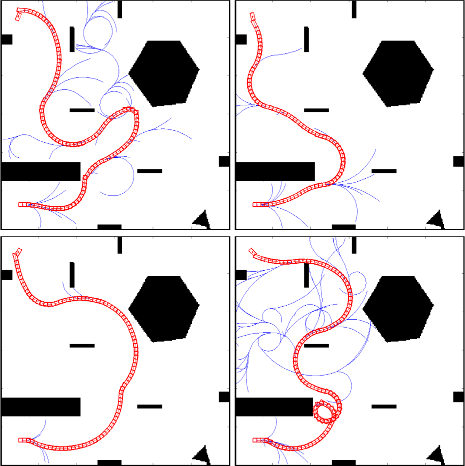
Under the control-based nonholonomic fast marching square, the FM² second potential is used to calculate the gradient values OX and OY associated with each grid point. The result of this operation is the OXY vector field of the motion plan. The directions of the gradient vectors point away from the obstacles. They follow paths across the different environment points to converge on the goal point. The magnitude of the vectors can be used to determined the velocity of the car-like robot, and as such the gradient vectors can be used to move the robot forward. Figures 6 and 7 show a car-like robot drawn over the vector field of the gradient vectors.

Figure 6.

Movement of the vehicle on the vector field

Figure 7.

Detailed representation of the vector field

Car-like robots have a limited steering angle, causing them to move along paths of bounded curvature. In Figure 8, a car-like robot is presented where R is the centre of the rear axis as represented by its (x,y) coordinates. The angle θ is the car orientation with respect to the OX axis. For the specification of the motion problem, it is necessary to consider the following nonholonomic constraint:

Figure 8.

A car-like robot model

\dot{y} \cos θ - \dot{x} \sin θ = 0

Moreover, the car-like movement can be modelled with a unit length between the front and rear axes of the wheels as:

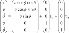
(\begin{matrix} \dot{x} \\ \dot{y} \\ \dot{θ} \\ \dot{v} \\ \dot{ϕ} \end{matrix}) = (\begin{matrix} v \cos ϕ \cos θ \\ v \cos ϕ \sin θ \\ v \sin ϕ \\ 0 \\ 0 \end{matrix}) + (\begin{matrix} 0 \\ 0 \\ 0 \\ 1 \\ 0 \end{matrix}) v_{1} + (\begin{matrix} 0 \\ 0 \\ 0 \\ 0 \\ 1 \end{matrix}) v_{2}

(4)

where the front wheel's orientation is expressed by φ, the car velocity by v̇, and the two control inputs are v₁,v₂, namely the acceleration of the robot and the front wheel's angular velocity.

This model can be expressed as a constraint on the curvature radius of the path. This constraint can be directly included in the algorithm using the vector field in the form of limits during the path calculation. It is interesting to note that the variables in Equation 4 are given by the vector field, except for the control inputs v₁ and v₂. This means that these control inputs can be easily deduced, and in this way the method not only gives the trajectory but also the control inputs to follow that trajectory. In Figure 9, an example of the φ variable over a trajectory is presented. It can be appreciated how the angle in the radians fluctuates between 0 and 2π over time. The dynamic of the car-like robot, in Equation 1, is used to find the variable u necessary to ensure the control. Since the method provides the positions, the velocities and the vector field, the control can be calculated. Equation 1 can be solved for the control u_i. In Figure 10, the resultant control signal for a motion plan example is shown.

Figure 9.

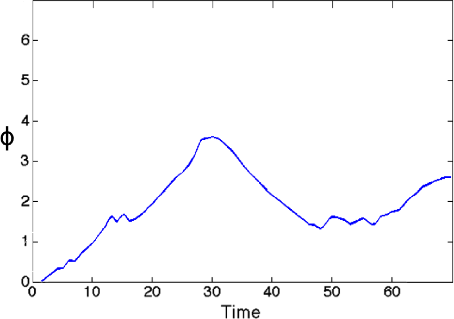
The front wheel's orientation φ vs. time for an example of car-like robot path planning

Figure 10.

The control signal u vs. time for an example of car-like robot path planning

In order to compute the complete path from the start to the goal position and orientation, the path is incrementally generated, beginning from the initial pose and according to the following order:

The front wheels are aligned with the vector field in the midpoint of the front axis.

The perpendicular lines to the front and rear wheels are considered and their intersection is taken as the centre of the step movement.

With the previously calculated centre C, the vehicle is moved a circumference arc of length proportional to the vector modulus corresponding to that point.

The previous process is repeated from the new point until the destination point is reached. The final point and orientation are always reached because the funnel potential ends at this point and orientation. Finally, the control inputs for the robot can be computed for the whole trajectory. Figure 11 shows the result of applying the algorithm for a parking manoeuvre.

Figure 11.

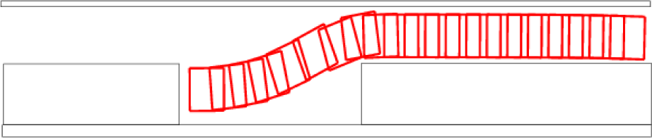
A parking manoeuvre using control-based FM²-NH

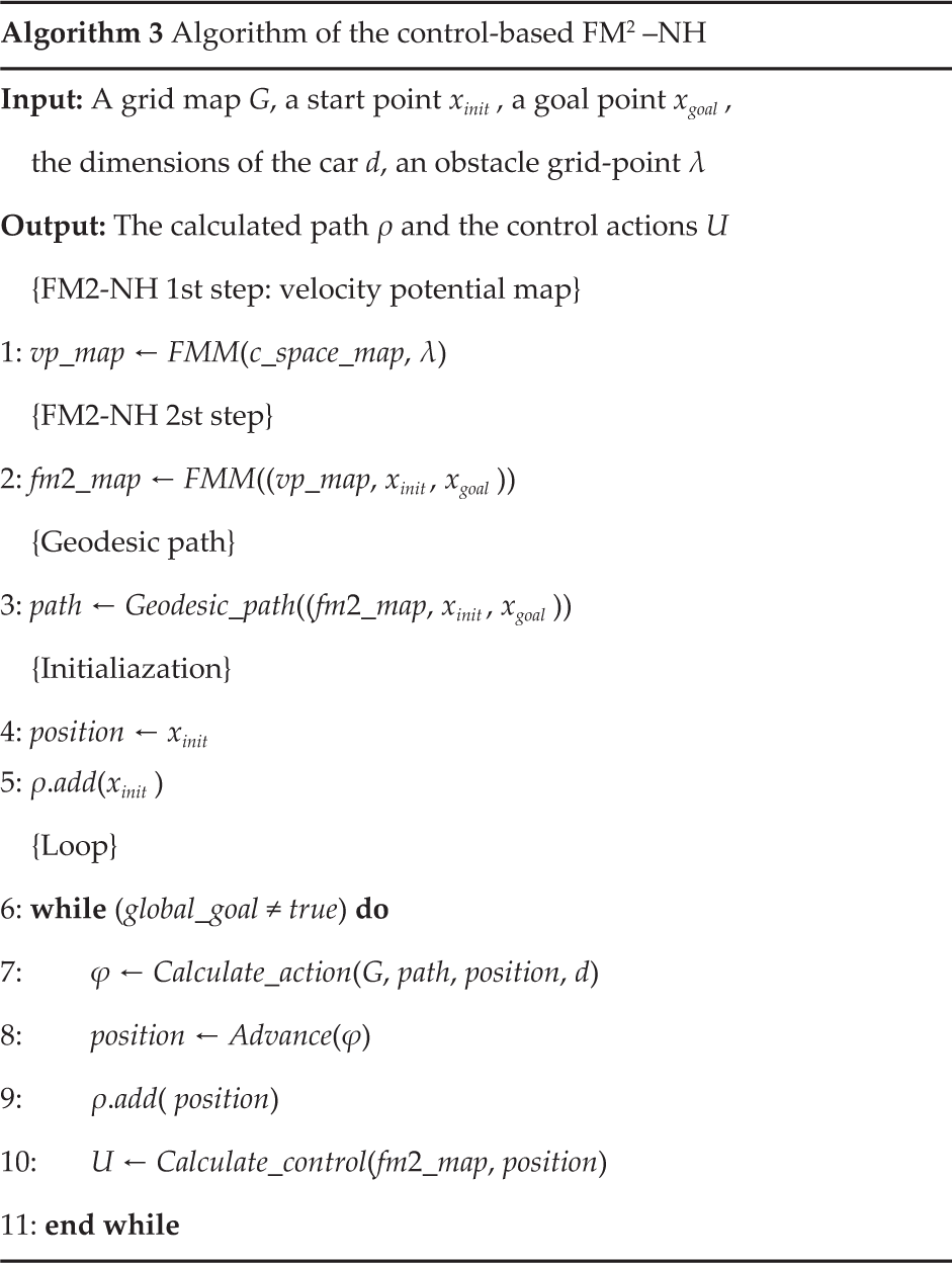
In Algorithm 3, the control-based FM2-NH approach is presented in pseudo-code.

The result of four examples generated with the control-based FM²-NH can be observed in Figure 12. The location and orientation for the start and goal points were randomly chosen. The presented map represents a cluttered environment frequently used to test RRT algorithms. The results of the experiments are discussed in the following Section 4.

Figure 12.

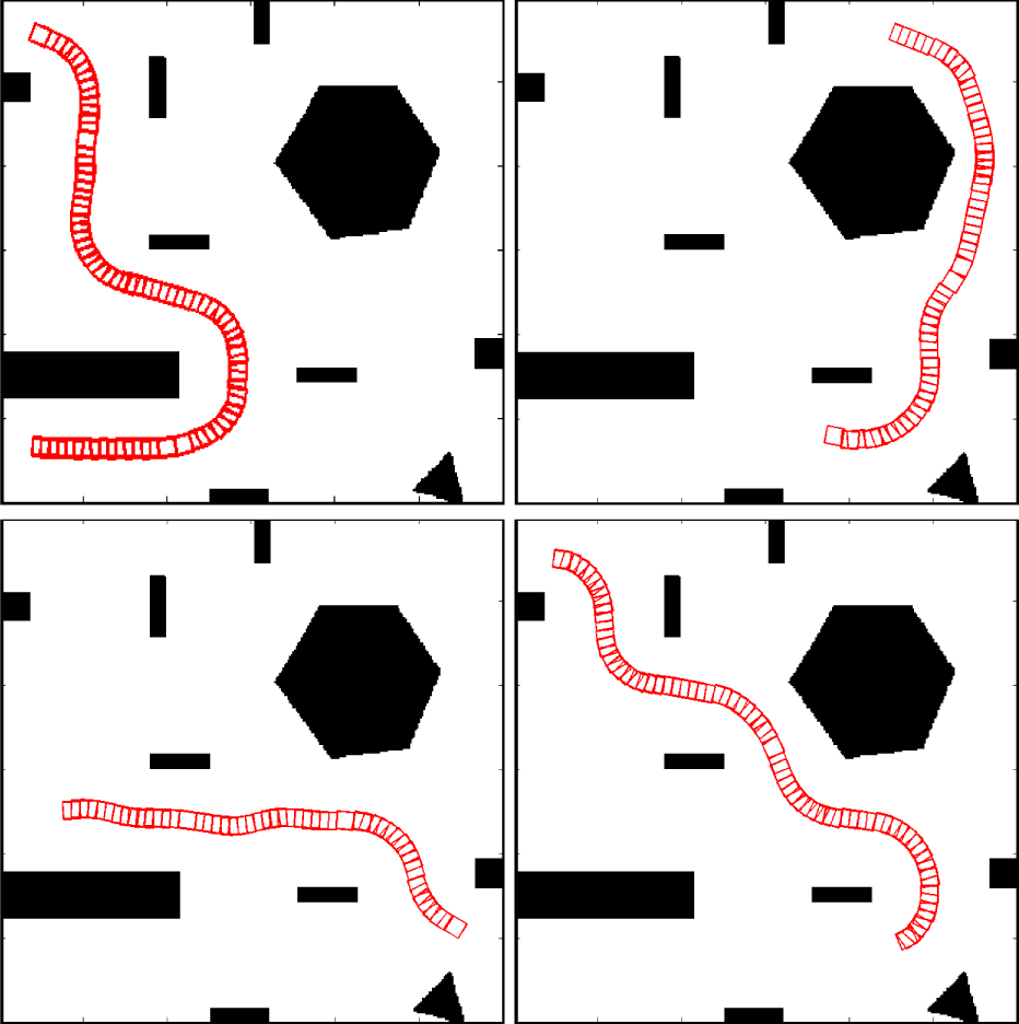
Different motion trajectories obtained with control-based FM²-NH

4. Results

In order to test the performance of the method and show its versatility, this section presents several experiments and benchmarking results. In Figure 12, four paths are generated using the control-based FM²-NH with different initial and goal positions and orientations. It can be appreciated from the four scenarios in Figure 12 that the obtained trajectories are smooth and safe from the start to the goal locations, and in this way the requirements of a good trajectory are fulfilled. The velocity potential field is shown in Figure 6. For a better view of the details, the image has been enlarged and the vectors have been normalized. A close-up of the Figure is presented in Figure 7. The methodology exhibits desirable features and versatility, generating trajectories that work properly for car-like robots.

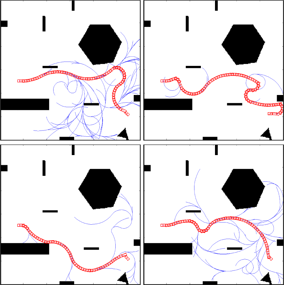
In Figure 13, the same four scenarios of Figure 12 are shown. On this occasion, the paths are generated using the C-space FM²-NH. The obtained trajectories are smooth and safe from the start to the goal location, and the results are very similar to those obtained using the control-based FM²-NH method.

Figure 13.

Different motion trajectories obtained with C-space FM²-NH

Different RRT paths are presented in Figures 14, 15, 16 and 17. Each of these RRT figures matches Figure 14 with regards to the initial and the goal points (including the orientation). Figure 14 matches its objectives with Figure 12's upper left FM²-NH path. Figure 15 has the same objectives as Figure 12's upper right FM²-NH path. Figure 16 matches those objectives of Figure 12's lower left FM²-NH path. Finally, Figure 17 has the same objectives as Figure 12's lower right FM²-NH path. As appreciated in the Figures, the FM²-NH methodology outperforms the quality of the paths generated with the RRT-NH method. From a visual inspection, the FM²-NH-generated paths seem safer, smoother and shorter. These suspicions will be discussed in the next section, where benchmarking parameters for path planners will be introduced.

Figure 14.

Motion trajectories obtained with RRT-NH for the first experiment

Figure 15.

Motion trajectories obtained with RRT-NH for the second experiment

Figure 16.

Motion trajectories obtained with RRT-NH for the third experiment

Figure 17.

Motion trajectories obtained with RRT-NH for the fourth experiment

4.1 Comparison of methods and benchmarking

The common limitation of all the reactive navigation methods is that they cannot guarantee global convergence on the goal location because they use only a fraction of the information available (the local sensory information). Some researchers have worked on introducing global information to the reactive collision avoidance methods to avoid local trap situations. This approach has been adopted by Ulrich [30] and uses a look-ahead verification to analyse the consequences of a given motion a few steps in advance in order to avoid trap situations. Other authors exploit the information about global environment connectivity to avoid trap situations (Minguez [31]). Those solutions still maintain the classical two-level approach, and require additional complexity at the obstacle avoidance level to improve the reliability at this level. The proposed method is consistent at the local and global scales because it guarantees a motion path (if it exists), and it does not require global replanning supervision to restart the planning when a local trap is detected or a path is blocked. Furthermore, the path calculated exhibits good safety and smoothness characteristics.

Most of the other methods give paths that are not smooth, even though they only provide a few loose points united by segments of straight lines. The only methods that give comparable results are based on harmonic functions (the solutions of Laplace's equation), but they have the problem of slowness.

Rapidly-exploring Random Trees (RRT): RRT is suited for high-degrees of freedom. It works well with six or seven degrees of freedom as regards computational time because it generates paths with a quick response, but the additional complexity supplied by the nonholonomic approach makes RRT function less effectively. Our method has not been tested with higher degrees of freedom, but for the problem addressed in this work (three-dimensions) good results are obtained, as set out in this section.

Figure 18 shows two different simulations. On the left-hand side, the trajectory generated by the fast marching-NH is clearly shorter than that calculated by the RRT on the right-hand side. The limitations of the RRT are specially important in this example, where the results obtained are very poor. We can illustrate that further comparisons with Figures 12, 14, 15, 16 and 17.

Figure 18.

Trajectories with control-based FM²-NH (left) and R RT-NH (right)

In order to provide metrics for the quality of the methods, the computational time, path length, smoothness and clearance-planning parameters are introduced below:

Computational times: The execution time is computed for each stage of the planning method, whether the algorithm is calculating a path or else optimizing in some way an already generated path.

Path length: This parameter is the sum of the distances from one way point to the next in the planner state space. For instance, the results presented here correspond to a two-dimensional space where the sum of the Euclidean distances between consecutive waypoints is an appropriate metric. Regarding benchmarking, the path length is usually connected to the method of performance, since a shorter path could represent a gain in energy and time. Nevertheless, this is not always necessarily true because the clearance - and hence the safety - can be notoriously affected when the path is the shortest possible.

Path smoothness: The smoothness of a path refers to the amplitude of the angles that are described while the robot follows the trajectory. Concerns arise when the robot's turning control is limited to a certain angle. Even when the mobile robot's base is holonomic, and thus capable of turning in an direction, small angles require less energy for their execution. Furthermore, when the path is performed in the real robot, smooth trajectories are more human friendly since they are more predictable, and rough paths seem unpredictable and violent when turning. In [32], a “generic infrastructure for benchmarking motion lanners” is presented and, in particular, an equation to measure the smoothness (denoted by κ) is proposed:

κ^{'} = \frac{1}{n} \sum_{i = 2}^{n} α_{i}^{2},

(5)

where α_i represents the angle between two consecutive segments of a path with n segments.

Clearance: This metric is related to the distance from the trajectory points to the closest obstacle, and it is determined by the average of the path points' clearances. It has also been defined in [32]:

μ_{c} = \frac{1}{n} \sum_{i = 1}^{n} δ_{i},

(6)

where δ_i represents the Euclidean distance from the point i of the path to the closest obstacle and n is the number of points of the path.

Success rate: This is equal to the percentage of times an algorithm is able to find a valid solution. Since the FM 2 - NH planner is a deterministic algorithm, it will always find a solution so long as it exists.

Box plots are used to present the benchmarking results in order to make a comparison between the FM²-NH and the RRT-NH planners. In the plots, the central band inside the box is the median. The bottom and top of the box define the first and third quartiles. The ends of the whiskers represent the most extreme points not considered outliers. The outliers are plotted with red crosses when necessary.

Over 25 experiments were conducted for each of the presented methods. The benchmarking parameters were calculated for all of them. The box plots in Fig. 19 show the computational time required by both the the RRT-NH and the control-based FM²-NH methods in order to calculate a path. It can be appreciated that the time needed by the control-based FM²-NH is much lower than the time required by the RRT technique to generate a path. The FM²-NH needs milliseconds to obtain results, while the median time of the RRT algorithm is around 15.1 seconds. As a consequence, our approach is able to recompute new trajectories very quickly, so that changes in the goal point can be addressed.

Figure 19.

Computational time benchmarks for RRT-NH and the control-based FM²-NH method

In Figure Fig. 20, the computational time required by the RRT-NH is now compared with the C-space FM²-NH approach. In this benchmark, the time of the FM²-based method increased to seconds. However, the time of the C-space FM²-NH was much lower than that of the RRT-NH. The C-space FM²-NH needs in median of 3.63 seconds of computational time.

Figure 20.

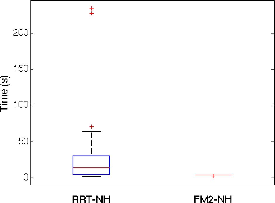
Computational time benchmarks for RRT-NH and the C-space F M²-NH method

In Figures 21 and 22, the ratio FM²-NH/RRT-NH is the variable used to compare both methods. In this Figure, the rest of the benchmarking parameters (path length, smoothness k ‘, and clearance μ_c) are analysed. The same configurations - the initial and goal locations and orientations - were taken. In the case of the path length, ratios smaller than one would indicate that the FM²-NH is better. For the smoothness and clearance, higher ratios mean that the FM²-NH is superior.

Figure 21.

Path length, smoothness and clearance benchmarks for the ratio of RRT-NH divided by the control-based FM²-NH

Figure 22.

Path length, smoothness and clearance benchmarks for the ratio RRT-NH divided by the C-space FM²-NH

In Figure 21, it can be observed that the path length ratio is smaller than one. This means that the length of the paths generated with the control-based FM²-NH are smaller in the median than those of RRT-NH. It should be noticed that, for these examples, the velocity potential map was not saturated, which means that the length of the FM²-NH approaches can be further reduced.

The smoothness ratio in Figure 21 approximates to one. Therefore, the paths are similar in smoothness. This result was expected because the nonholonomic restrictions prevent the planners from taking pronounced turns. Under the regular RRT method, the angle of the turns tends to be more violent. Finally, the clearance ratio is greater than one, showing a significant advantage for the control-based FM²-NH over RRT-NH. Naturally, this was to be expected since the RRT methods do not consider safety measures in their implementation; meanwhile, the FM²-based methods intrinsically include this parameter through the velocity potential map. In Figure 22, very similar benchmarking results were obtained for the C-space FM²-NH. Both approaches generate consistent trajectories with desirable properties.

An additional advantage of the obtained implementation is the ease of including, through the velocity potential map, other constraints such as uneven terrains, slopes, friction, winds or currents (in the case of underwater applications).

5. Conclusion

The motion planning approaches presented in this document are based on FM². They are both able to generate trajectories of high quality for nonholonomic mobile robots, i.e., with smoothness and clearance.

Simulations and experiments evidenced how the C-space and the control-based FM²-NH outperform the RRT-NH planner results. In the current study, comparing the FM²-NH methods showed that they generate considerably shorter paths in length, and that trajectories are more secure and smooth. Due to its random nature, the RRT-NH planner exhibits several loops in the trajectories which produce longer paths; on the other hand, the deterministic quality of the FM² method (inherited by our methods) not only produces more coherent paths without loops, but also guarantees the computation of a solution if it exists, a criteria that is not met by RRT-NH or probabilistic planners.

The computational complexity for the FMM, as well as for its successor, the FM², is defined as linear O(n), where n is the number of grid points in the environment map. Since the proposed method is based on the later method, the FM2-NH methods are also highly efficient with a linear runtime complexity of O(n).

The FM²-NH makes several noteworthy contributions to path planning. Nevertheless, the most remarkable is that the algorithms calculate not only good paths but also provide the control variables needed to execute these trajectories.

Future work will include combining both solutions and introducing some changes to make it possible to use them for dynamic environments.

Footnotes

6. Acknowledgements

This work is funded by project number DPI2010-17772, by the Spanish Ministry of Science and Innovation, and also by the RoboCity2030-II-CM project (S2009/DPI-1559), funded by Programas de Actividades I+D en la Comunidad de Madrid, and co-funded by the Structural Funds of the EU.

References

Adams

Breazeal

Brooks

RA.

, and Scassellati

Humanoid robots: A New kind of tool. IEEE Intelligent Systems, 15(4):25–31, July 2000.

Borenstein

and Koren

The vector field histogram-fast obstacle avoidance for mobile robots. IEEE Transactions on Robotics and Automation, 7(3): 278–288, June 1991.

Moravec

and Elfes

High resolution maps from wide angle sonar. In Proceedings. 1985 IEEE International Conference on Robotics and Automation, volume 2, pages 116–121. Institute of Electrical and Electronics Engineers, March 1985.

Latombe

Jean-Claude

. Robot Motion Planning. Kluwer Academic Publishers, Norwell, MA, USA, July 1991.

LaValle

Steven Michael

. Planning Algorithms. Cambridge University Press, 2006.

Conner

David C.

Rizzi

Alfred A.

, and Choset

Howie

. Integrated planning and control for convex-bodied nonholonomic systems using local feedback control policies. In Proceedings of Robotics: Science and Systems, Philadelphia, 2006.

Conner

David C.

Kress-Gazit

Hadas

Choset

Howie

, and Rizzi

Alfred A.

Valet parking without a valet. In IEEE/RSJ International Conference on Intelligent Robots & Systems, 2007.

Lozano-Perez

Spatial Planning: A Configuration Space Approach. IEEE Transactions on Computers, C-32(2):108–120, February 1983.

Kiss

Domokos

and Tevesz

Gábor

. Nonholonomic Path Planning for a Point Robot with Car-Like Kinematics. Periodica Polytechnica Electrical Engineering, 57(3):65, August 2013.

10.

Lafferriere

and Sussmann

H. J.

Motion Planning For Controllable Systems Without Drift. In Proceedings of the IEEE International Conference on Robotics and Automation, pages 1148–1153, 1991.

11.

Murray

R.M.

and Sastry

S.S.

Nonholonomic motion planning: Steering using sinusoids. IEEE Transactions on Automatic Control, 38(5):700–716, May 1993.

12.

Sekhavat

and Laumond

J.-P.

Topological property for collision-free nonholonomic motion planning: The case of sinusoidal inputs for chained form systems. IEEE Transactions on Robotics and Automation, 14(5):671–680, 1998.

13.

Fliess

Michel

Lévine

Jean

, and Rouchon

Pierre

. Flatness and defect of nonlinear systems: Introductory theory and examples. International Journal of Control, 61:1327–1361, 1995.

14.

Kavraki

L.E.

Svestka

Latombe

J.-C.

, and Overmars

M.H.

Probabilistic roadmaps for path planning in high-dimensional configuration spaces. IEEE Transactions on Robotics and Automation, 12(4): 566–580, 1996.

15.

LaValle

Steven Michael

. Rapidly-Exploring Random Trees A New Tool for Path Planning. Technical report, Iowa State University, 1998.

16.

Laumond

J.-P.

Jacobs

P.E.

Taix

, and Murray

R.M.

A motion planner for nonholonomic mobile robots. IEEE Transactions on Robotics and Automation, 10(5):577–593, 1994.

17.

Sekhavat

and Chyba

Nonholonomic deformation of a potential field for motion planning. In Proceedings 1999 IEEE International Conference on Robotics and Automation (Cat. No.99CH36288C), volume 1, pages 817–822. IEEE, 1999.

18.

LaValle

and Kuffner

Jr . Rapidly-exploring random trees: Progress and prospects. Technical report, Iowa State University, 2000.

19.

Garrido

Santiago

Moreno

Luis

Blanco

Dolores

, and Martin

Fernando

. FM2: A Real Fast Marching sensor-based Motion Planner. In 2007 IEEE/ASME international conference on Advanced intelligent mechatronics, pages 1–6, 2007.

20.

Dijkstra

E. W.

A Note on Two Problems in Connexion with Graphs. Numerische Mathematik, 1(1): 269–271, December 1959.

21.

Hart

Peter

Nilsson

Nils

, and Raphael

Bertram

. A Formal Basis for the Heuristic Determination of Minimum Cost Paths. IEEE Transactions on Systems Science and Cybernetics, 4(2):100–107, 1968.

22.

Cohen

Laurent D.

and Kimmel

Ron

. Global Minimum for Active Contour Models: A Minimal Path Approach. International Journal of Computer Vision, 24(1):57–78, August 1997.

23.

Sethian

J. A.

Level Set Methods and Fast Marching Methods: Evolving Interfaces in Computational Geometry, Fluid Mechanics, Computer Vision, and Materials Science. Cambridge University Press, 1999.

24.

Garrido

and Moreno

. FM2: A Real-time sensor-based feedback controller for mobile robots. International Journal of Robotics and Automation, 24(1): 48–65, 2009.

25.

Garrido

Santiago

Moreno

Luis

Javier

, and Pedro

General Path Planning Methodology for Leader-Follower Robot Formations. International Journal of Advanced Robotic Systems, page 1, January 2013.

26.

Arismendi

Cesar

Martin

Fernando

Garrido

Santiago

, and Moreno

Luis

. Smooth anytime motion planning using Fast Marching. In Eurocon 2013, pages 1972–1979. IEEE, July 2013.

27.

Gómez

Javier V.

Vale

Alberto

Garrido

Santiago

, and Moreno

Luis

. Performance analysis of fast marching-based motion planning for autonomous mobile robots in ITER scenarios. Robotics and Autonomous Systems, October 2014.

28.

Sethian

and Vladimirsky

. Ordered upwind methods for static Hamilton–Jacobi equations: Theory and algorithms. SIAM Journal on Numerical Analysis, 2003.

29.

Valero-Gomez

Alberto

Gomez

Javier V.

Garrido

Santiago

, and Moreno

Luis

. The Path to Efficiency: Fast Marching Method for Safer, More Efficient Mobile Robot Trajectories. IEEE Robotics & Automation Magazine, 20(4):111–120, December 2013.

30.

Ulrich

and Borenstein

VFH*: Local obstacle avoidance with look-ahead verification. In Proceedings 2000 ICRA. Millennium Conference. IEEE International Conference on Robotics and Automation. Symposia Proceedings (Cat. No.00CH37065), volume 3, pages 2505–2511. IEEE, 2000.

31.

Minguez

Montano

Simeon

, and Alami

Global nearness diagram navigation (GND). In Proceedings 2001 ICRA. IEEE International Conference on Robotics and Automation (Cat. No.01CH37164), volume 1, pages 33–39. IEEE, 2001.

32.

Cohen

Benjamin

Sucan

Ioan A.

, and Chitta

Sachin

. A generic infrastructure for benchmarking motion planners. In 2012 IEEE/RSJ International Conference on Intelligent Robots and Systems, pages 589–595. IEEE, October 2012.

Nonholonomic Motion Planning Using the Fast Marching Square Method

Abstract

Keywords

1. Introduction

2. Fundamentals of the Method

2.1 Fast Marching and Path Planning

2.2 Implementation

2.3 Fast Marching Square

3. Fast Marching Square Applied to Nonholonomic Car-like Robots

3.1 Nonholonomic Fast Marching Square in C-space

3.2 Control-based Nonholonomic Fast Marching Square

4. Results

4.1 Comparison of methods and benchmarking

5. Conclusion

Footnotes

6. Acknowledgements

References