Sage Journals: Discover world-class research

Abstract

Currently, industrial robotic manipulators are applied in many manufacturing applications. In most cases, an industrial environment is a cluttered and complex one where moving obstacles may exist and hinder the movement of robotic manipulators. Therefore, a robotic manipulator not only has to avoid moving obstacles, but also needs to fulfill the manufacturing requirements of smooth movement in fixed tact time. Thus, this paper proposes a virtual velocity vector-based algorithm of offline collision-free path planning for manipulator arms in a controlled industrial environment. The minimum distance between a manipulator and a moving obstacle can be maintained at an expected value by utilizing our proposed algorithm with established offline collision-free path-planning and trajectory-generating systems. Furthermore, both joint space velocity and Cartesian space velocity of generated time-efficient trajectory are continuous and smooth. In addition, the vector of detour velocity in a 3D environment is determined and depicted. Simulation results indicate that detour velocity can shorten the total task time as well as escaping the local minimal effectively. In summary, our approach can fulfill both safety requirements of collision avoidance of moving obstacles and manufacturing requirements of smooth movement within fixed tact time in an industrial environment.

Keywords

Robotic manipulators Moving obstacles Virtual velocity vector Collision-free path planning Detour velocity

1. Introduction

Industrial robotic manipulators are commonly used to complete various tasks in manufacturing plants. In a dynamic industrial environment, there are moving obstacles such as AGVs, parts on the conveyor, overhead cranes or other robotic manipulators. This means that the working space of a manipulator is constrained. On the one hand, a robotic manipulator has to avoid moving obstacles in consideration of safety requirements. On the other hand, it needs to fulfill the manufacturing requirements of working speed, positioning accuracy and smoothness of movement within tact time. Therefore, this paper proposes a virtual velocity vector-based algorithm and establishes corresponding offline collision-free path-planning and trajectory-generating systems. As a result, the minimum distance between a manipulator and a moving obstacle is maintained at the expected value while time-efficient, continuous and smooth task space paths and joint space trajectories are generated which can satisfy the requirements of real manufacturing applications.

The majority of collision-free path-planning algorithms for robotic manipulators can be classified into three categories.

The first approach is to use the collision map. This method generally assumes a moving robot or obstacle with higher priority moving along a predefined path, which the other robots with lower priority should avoid through waiting or speed modification, preventing the path searching from entering the collision areas on the collision map. This approach is based on geometry calculation with decent visualization of the collision map and is applied in collision avoidance of mobile robots [1], planner articulated manipulators [2] and six-degrees of freedom (DoF) manipulators [3–5].

An alternative method for collision avoidance of manipulators is to transform obstacles from task space to configuration space (C-space) and then to map a valid path within the configuration space. This method is generally utilized with robot arms rather than mobile robots, such as planner articulated manipulators [6–8] or three-DoF [9]/six-DoF robot arm [10] avoiding fixed obstacles, and collision-free path planning between articulated robot arms [8,11].

The third possible approach is the potential field-based method, usually called artificial potential field (APF) [12] or virtual force field (VFF) [13]. The establishment of APF/VFF is simple and fast, which makes it popular for collision-free path planning of mobile robots [14,15] and articulated manipulators [12,16,17]. The APF/VFF approach is a force-actuated method that assumes there are two types of potential field/force applied on a robot, namely attractive potential field/virtual force and repulsive potential field/virtual force, with active regions around each obstacle. The attractive potential field/virtual force is active and constantly applied on the robot towards the goal, while the repulsive potential field/virtual force is only activated when the robot enters the obstacle's active region. The robot is actuated towards the destination by the superimposed force of both types of potential field/virtual force while the robot avoids the obstacles on the path.

Although the APF/VFF approach is simple and fast, with this approach robot dynamics usually need to be considered and the torque control mode employed for joint servomotors. Commercial industrial robotic manipulators rarely provide torque control mode [18] but actuate the joints instead by position or velocity signal. For this reason, some researchers have used the potential field function to calculate correction of position in task space, utilizing robotic kinematics for robot control [19–21], Other researchers have constructed virtual velocity functions and utilized velocity control mode to actuate mobile robots [22–24] and articulated robot arms [25] in an environment with moving obstacles. Fn [26–28], the potential field function is used to calculate the correction of velocity in task space. The redundancy of planner multi-link robot arms is utilized to avoid obstacles or other robots. Bosscher P. and Wu P.W.et al. established virtual velocity function and utilized the Jacobin matrix for real-time collision-free path planning and motion control for six-DoF robotic manipulators [29, 30]. But another issue is that the potential field-based method may trap in local minimal [13] when attractive and repulsive forces confront each other on the same line; this is also termed as collinear condition [31]. Traditional methods for escaping local minimal include the wall-following method [32], simulated annealing [33], and modification of repulsive field function [34]. A tangential field has also been proposed and added to the repulsive field [13]. This tangential field helps the robot to detour around the obstacle. Similarly, Zeng L.Q. and Bone G.M. [31,35] used virtual tangential force to escape collinear condition, terming this virtual force “detour force”. Tangential field/detour force is a simple and direct method that performs perfectly in escaping local minimal [25,36].

The three methods described above are capable of providing collision avoidance of robotic manipulators. However, there are still various limitations for each method in practical applications. First, the collision map requires the robot to avoid obstacles by waiting or decreasing speed, which can only be effective when the path is known a priori and cannot be modified – this is invalid when the path is unknown or obstacles block the path. This deadlock problem was researched for a two-manipulator situation in [5]. Second, the C-space collision-free path lacks intuitive-ness, so it is more difficult to understand compared with the task-space path. The full construction of high-dimensional configuration space such as a six-DoF manipulator is complex and expensive, with complexity rising exponentially due to the increase of DoFs. Efficiency improvement of the C-space algorithm is researched in [6, 9], Finally, industrial robot arms equipped in manufacturing plants generally execute predefined repetitive motion in fixed tact time, and the manufacturing requirements of working speed, positioning accuracy and smoothness of movement need to be fulfilled. The force-actuated potential field-based method needs to deploy the torque control mode of joint motors when it is applied on articulated manipulators [12, 13, 16, 17], but the accuracy of torque control mode highly relies on the accuracy of the dynamics equation – this is difficult to achieve with industrial manipulators working in severe environments. Additionally, operators are required to understand robot dynamics. As a result, the position or velocity-actuated potential field-based method is far preferable in satisfying the requirements of high speed and positioning accuracy in manufacturing applications.

The real-time/online collision avoidance technologies of manipulators [12, 17, 28 –30] calculate and generate the paths and joint trajectories in real time, but the shape, length, and destination of path and total task time are indeterminate, so it is impossible to guarantee the repetitive positioning accuracy and tact time. Even more, the online-generated trajectory is not smooth and optimal, such that the joint velocity may suddenly change or reach the upper/lower limits, which may result in oscillation or unstable movement. Therefore, offline and optimized path-planning and trajectory-generating approaches are more appropriate for industrial manipulators executing rapid and repetitive work with high positioning accuracy.

In summary, based on the safety requirements of collision avoidance and manufacturing requirements of working speed and smoothness of movement in reality, this paper presents a virtual velocity vector-based method with corresponding collision-free path-planning and trajectory-generating systems for six-DoF industrial manipulators, which is based on existing artificial potential field and virtual velocity methods, in controlled industrial environments with moving obstacles. The tool-end velocities of manipulators and velocities of moving obstacles are assumed to be constant and known. Our proposed method has the following advantages.

Smoothness of movement: velocities of trajectories are continuous and smooth, both in joint space and Cartesian space, which can eliminate oscillation. Generated discrete joint position signals are easily executed repeatedly on industrial robotic manipulators.

Safety: the minimum distance (safe distance) between a manipulator and a moving obstacle can be specified manually and maintained steadily at the expected value during the task.

Escaping local minima: The problem of trapping in local minima for manipulators in a 3D environment is addressed by the proposed “detour velocity” with the calculating principles of its directional vector.

Time efficiency: Task time can be reduced to expected tact time simply by increasing the only coefficient of “detour velocity”.

The organization of this paper is as follows. In Section 2, the method for establishing the bounding box model of a six-DoF industrial manipulator is explained. The virtual attractive and repulsive velocity functions are designed in Section 3 together with the improvement of functions. The offline collision-free path-planning and trajectory-generating systems are presented in Section 4. In Section 5, the determination of the directional vector of detour velocity for escaping local minimal in a 3D environment is described, and an updated repulsive velocity function with detour velocity is presented. The simulations are done in section 6, with a discussion of the results. Finally, we end with conclusions and discussion of future work in section 7.

2. Establishment of the bounding box model

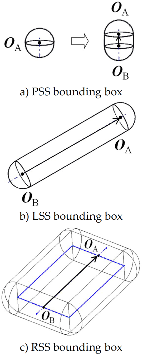
The geometry of the manipulators and obstacles in reality is complex; therefore, before we start to design the virtual attractive and repulsive velocity functions for the manipulator avoiding moving obstacles, it is important to construct the bounding box representation and choose the algorithm of collision detection and distance calculation. Swept Sphere Volumes (SSV) bounding box representation together with a distance calculation algorithm [37], which is popular in polyhedron approximation, is chosen in this paper since it is a simple and systematic method with a good balance between cost and accuracy. It is suitable for robot arm modelling [5]. There are three basic bounding boxes of SSV: Point Sphere Volumes (PSS), Line Sphere Volumes (LSS) and Rectangular Sphere Volumes (RSS) [38], as shown in Figure 1. These are related to the point, line and rectangular feature, respectively. The SSV algorithm is a feature-based algorithm that computes the distances between a pair of features. The distance between two bounding boxes is equal to the distance between two features minus the radius of each bounding box. We will not explain this method in detail, but refer readers to [37, 38] for a systematic overview.

Figure 1.

Three geometry primitives of SSV bounding box [37]

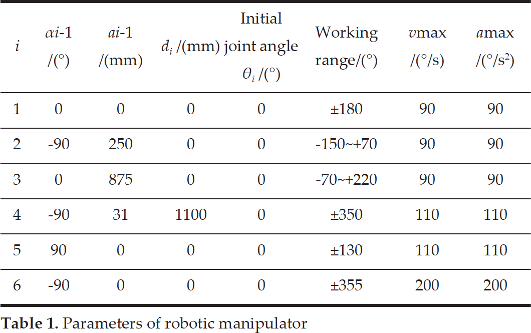
The robotic manipulator model employed in this paper is illustrated in Figure 2 a); the link parameters, joint angle, velocity and acceleration limits are shown in Table 1. The length of the manipulator's end tool is 210 mm. The whole manipulator is divided and represented by 12 bounding boxes with the unit number, as displayed in Figures 2 b) and c). The arrows on the bounding boxes are related to the detour velocity calculation, which will be explained in section 5.

Figure 2.

Models of manipulator and bounding boxes

The virtual velocity function introduced in section 3 utilizes the Jacobian relationship of serial manipulators. The corresponding “partial Jacobian matrix” [29] depends on which robot link is located in the closest point, and will be explained in section 4. Therefore, the 12 bounding boxes are classified into three categories as follows and a three-link model is established. The units of the bounding boxes are illustrated in Figure 2.

Table 1.

Parameters of robotic manipulator

i	αi−1/(°)	ai−1/(mm)	d_i/(mm)	Working range/(°)	vmax/(°/s)	amax/(°/s²)
1	0	0	0	±180	90	90
2	−90	250	0	−150-+70	90	90
3	0	875	0	−70-+220	90	90
4	−90	31	1100	±350	110	110
5	90	0	0	±130	110	110
6	−90	0	0	±355	200	200

Link 1: Units 4, 5 and 6.

Link 2: Units 7, 8, 9 and 10.

Link 3: Units 11 and 12.

3 Virtual velocity vectors and control functions

In order to realize velocity-actuated movement of the manipulator while avoiding moving obstacles, the virtual velocity vectors and corresponding control functions are presented.

3.1 Virtual velocity vectors

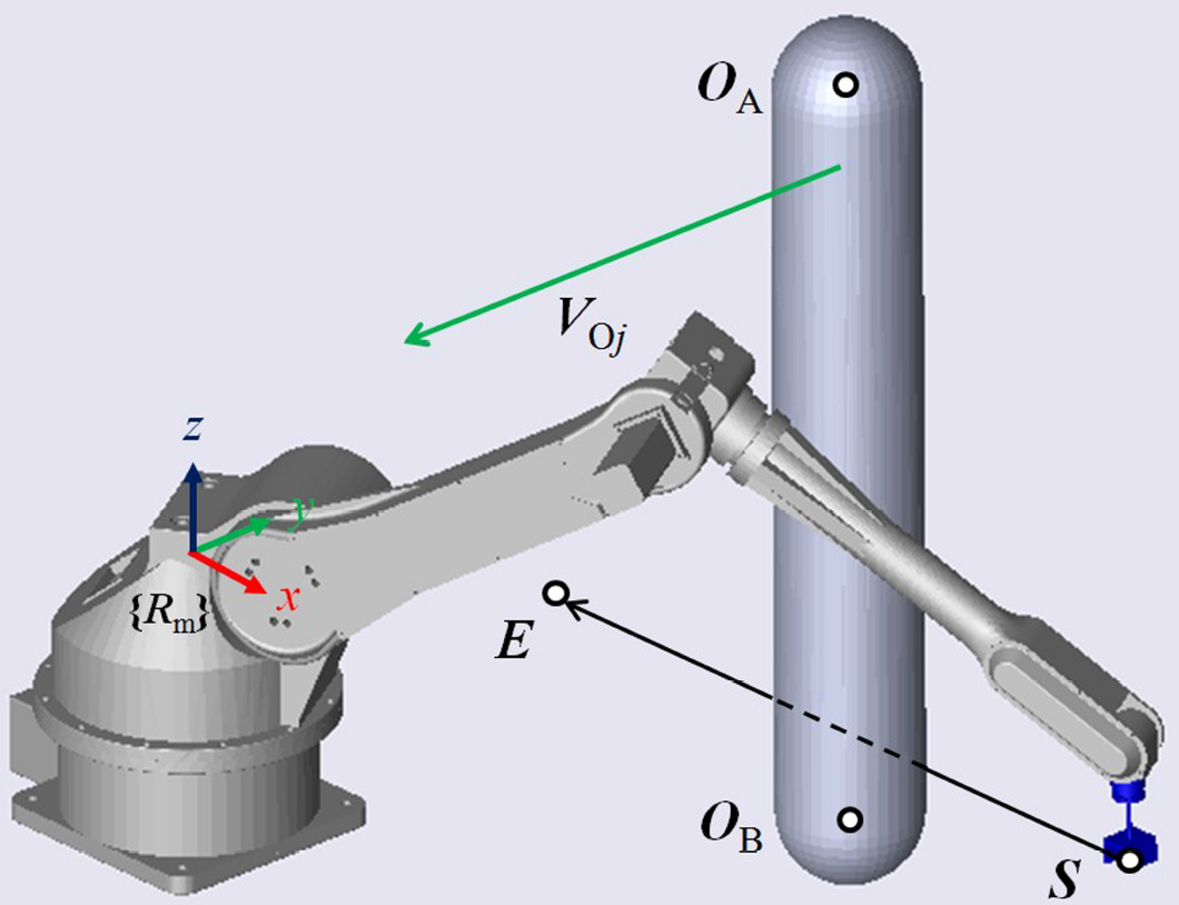
Virtual velocity vectors include virtual attractive and repulsive velocity vectors. There is an illustration of these two virtual velocity vectors for a manipulator M avoiding a moving obstacle O_j in Figure 3. The links and end tool of the manipulator are represented by LSS bounding boxes while the moving obstacle is represented by an RSS bounding box. The radii of each bounding box are r_M and r_Oj, respectively. D_j is the minimum distance between the manipulator and the obstacle. The base coordinate system of manipulator M is { K _m}, which is also the world coordinate system in most cases. The current position coordinate of the manipulator's tool end is T_M = (x_TM, y_TM) and the destination of the tool end is E=(x_E,y_E). The established manipulator and obstacle model, which are actuated by virtual velocity vector, are a discrete system with sampling interval t_s.

Figure 3.

Virtual attractive and repulsive velocity vector

Manipulator M is actuated towards the goal by the superimposed velocity of virtual attractive velocity vector V _att and repulsive velocity vector V _repj. Meanwhile, moving obstacle O_j is actuated by a virtual attractive velocity vector V _Qj. V _{att_M} and V _{Oj_n} are the approaching velocity vectors along the direction of D_j. To facilitate the description in the next section, it is assumed that v_{att_M}, v_repj and v_{Oj_n} are the corresponding velocity variables that indicate the magnitude of vectors V _{att_M}, V _repj and V _{Oj_n} along the direction D_j.

There are active regions outside each manipulator link or tool with a safety radius D_s. The virtual attractive velocity vectors V _att and V _Oj are active and are constantly applied on the manipulator tool end and the obstacle towards the goal. Meanwhile, the virtual repulsive velocity vector V _repj is only activated when the obstacle enters the robot's active region; in other words, V _repj is only activated when the minimum distance D_j < D_s.

M _j and P _j are a pair of closest points between the manipulator and moving obstacle in relation to the SSV algorithm in coordinate system { R _m}. M _j = (M_xj,M_yj), P _j=(P_xj,P_yj), D_j = ‖P_jM_j‖-r_M-r_Oj. ‖P_jM_j‖ is the norm of vector P _j M _j.

3.2 Design of control function

On the basis of the virtual velocity vector model established in section 3.1, the control functions of virtual attractive velocity and virtual repulsive velocity are designed and improved in this section.

3.2.1 Attractive velocity function

It is assumed that the tool end T _M of manipulator M is actuated towards the goal E with constant speed v_att. The virtual attractive velocity vector V _att is obtained by Eq. (1).

V_{att} = v_{att} \cdot T_{M} E / ‖ T_{M} E ‖

(1)

T _M E =(x_TM–x_E,y_TM–y_E), T _M E /‖ T _M E ‖ is the unit vector of V_attj.

3.2.2 Repulsive velocity function

The proposed repulsive velocity function Eq. (7) is a function of the minimum distance D_j and the approaching velocity D_j along the direction of D_j. ΔD_j and D_j indicate the position error and the approaching velocity along the direction of D_j, which are defined in Eqs. (2,3).

Δ D_{j} = D_{s} - D_{j}

(2)

{\dot{D}}_{j} = d D_{j} / d t

(3)

On the one hand, ${\dot{D}}_{j} < 0$ indicates the manipulator is approaching the obstacle. In this case, the effect of ${\dot{D}}_{j}$ is taken into consideration in the control function. On the other hand, ${\dot{D}}_{j} \geq 0$ suggests the manipulator is departing from the obstacle such that the effect of ${\dot{D}}_{j}$ is not considered; therefore, let ${\dot{D}}_{j}$ = 0 as defined in Eq. (4).

\begin{array}{l} {\dot{D}}_{j} = d D_{j} / d t, {\dot{D}}_{j} < 0 \\ {\dot{D}}_{j} = 0, {\dot{D}}_{j} \geq 0 \end{array}

(4)

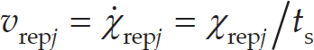
In order to maintain the minimum distance D_j between a manipulator and a moving obstacle at the expected value D_s, the control function of position modification χ_repj is designed and can be computed by Eq. (5) during sampling interval t_s. Moreover, the position modification during sampling interval t_s can be transformed into velocity modification by Eq. (6).

χ_{rep j} = k_{d} \cdot Δ D_{j} + k_{v} \cdot {\dot{D}}_{j} \cdot t_{s}

(5)

v_{rep j} = {\dot{χ}}_{rep j} = χ_{rep j} / t_{s}

(6)

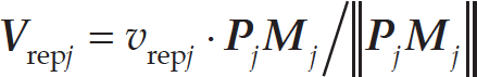
k_d and k_v are the proportional and differential coefficient, respectively. The repulsive velocity function can be computed by Eq. (7). P _j M _j / || P _j M _j || is the unit vector of V _repj. Notice that k_d = 1, k_v = −1.

\begin{array}{l} {\begin{matrix} v_{rep j} = 0. D_{j} > D_{s} \\ v_{rep j} = k_{d} \cdot Δ D_{j} / t_{s} + k_{v} \cdot {\dot{D}}_{j}, 0 < D_{j} \leq D_{s} \\ v_{rep j} = + \infty . D_{j} < 0 \end{matrix} \\ V_{rep j} = v_{rep j} \cdot P_{j} M_{j} / ‖ P_{j} M_{j} ‖ \end{array}

(7)

Finally, the synthesized virtual velocity function can be obtained based on V _att and V _repj, computed by Eqs. (1,7) with corresponding joint velocity calculated by Eq. (9).

V_{att}' = {[\begin{matrix} V_{att} & ω_{att} \end{matrix}]}^{T}, V_{rep j}' = {[\begin{matrix} V_{rep j} & ω_{rep j} \end{matrix}]}^{T}

(8)

\begin{matrix} {\dot{Θ}}_{rep j} = J_{^{rep j}}^{- 1} (Θ_{M}) \cdot V_{rep j}' \\ {\dot{Θ}}_{att} = J_{^{att}}^{- 1} (Θ_{M}) \cdot V_{att}' \end{matrix}

(9)

It is important to note that when multiple obstacles enter the active region of the manipulator simultaneously, the superimposed joint velocity modification is computed by Eq. (10).

{\dot{Θ}}_{rep} = \sum_{j = 1}^{n} {\dot{Θ}}_{rep j}

(10)

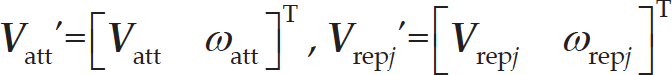
ω in Eqs. (8–10) expresses the angular velocity vector of manipulator tool end, ω_att is set according to the requirements of the task, and ω_repj can be set to (0,0,0) in Eqs. (8,9) if collision avoidance is conducted only by modifying the linear velocity vector. Finally, the synthesis of ${\dot{Θ}}_{att}$ and ${\dot{Θ}}_{rep}$ is sent to multiple joint motors as the joint velocity signal values.

In the case of a serial manipulator, J _att(Θ_M) is the Jacobian matrix of manipulator from tool end T _E to the robot base while J _repj(Θ_M) is a “partial Jacobian matrix” that only includes the joints between the closest point M _j and the robot base [29].

3.2.3 Verification of virtual repulsive velocity function

A step and a sine signal of approaching velocity are used for testing in order to verify the control performance of the minimum distance D_j of the proposed virtual repulsive velocity function in Eq. (7) when a moving obstacle enters the active region of the manipulator. T, t and t_s indicate time length of simulation, time variable and sampling interval when T=10s, t_s=0.2s and D_s=50 mm.

When the approaching velocity is a step signal (v_{att_M}+v_{Oj_n} = −150 mm/s), repulsive velocity function calculated in Eq. (7) can maintain the minimum distance between a manipulator and a moving obstacle at the expected value Dg, as plotted in Figure 4.

When the approaching velocity is a sine signal (v_{att_M}+v_{Oj_n} = | sin(πt/10) | (−150) mm/s), the repulsive velocity function cannot keep the minimum distance D_j between a manipulator and a moving obstacle at the expected value D_s, but drops below D_s, as Figure 5 shows.

Figure 4.

Response curve of D_j with step signal input

Figure 5.

Response curve of Dj with sine signal input

3.2.4 Modification to virtual repulsive velocity function

It is clear in Figure 5 that when the approaching velocity is a sine signal (v_{att_M}+v_{Oj_n} = | sin(πt/10)|(−150) mm/s), the repulsive velocity function fails to maintain the minimum distance D_j at expected value D_s. The reason for this is that the magnitude of $\dot{D}$ calculated by Eq. (4) is smaller than the true value of approaching velocity (v_{att_M}+v_{Oj_n}) if D_j≤D_s for two adjacent sampling intervals. Smaller D produces insufficient repulsive velocity. A modification is made to address this issue of Eq. (4). The new variable ${\dot{D}}_{r}$ is defined and used to save the true value of approaching velocity (v_{att_M}+v_{Oj_n}) between the manipulator and the moving obstacle. ${\dot{D}}_{r}$ is computed by Eq. (11), which is a supplement to Eq. (4); that is, $\dot{D}$ is calculated by Eq. (4) originally and after the modification by Eq. (4) plus Eq. (11).

{\dot{Θ}}_{rep} = \sum_{j = 1}^{n} {\dot{Θ}}_{rep j}

(11)

In addition, in Eq. (11), there are four magnitude combinations between D_j and D_s. Only if D_jD_s for two adjacent sampling intervals, is the modification made. D_j(t-1) is defined as the minimum distance at last time moment t−1, while D_j is still that at time moment t.

k_r is a coefficient that needs to be set according to the maximum changing rate of approaching velocity: the greater the maximum rate of change, the larger k_r should be. In this section, k_r is set to 2. On the one hand, for step signal input of approaching velocity, the response curve of D_j is the same as in Figure 4. On the other hand, for sine signal input of approaching velocity, the response curve of Dj is as displayed in Figure 6. Graphically, after the modification, the error adjustment of minimum distance D_j can be figured out precisely by repulsive velocity function Eq. (7). The minimum distance D_j is maintained steady at expected value D_s.

Figure 6.

Response curve of Dj after modification

However, coefficient k_r is generally unknown in advance in reality. One possible approach to determine k_r is to set an estimated value (e.g., k_r=1) in advance and to increase the value until the response curve of D_j is satisfied.

4 Offline collision-free path-planning and trajectory-generating systems

The industrial articulated manipulator needs to fulfill not only the safety requirements of collision avoidance, but also the manufacturing requirements of smooth movement in fixed tact time. To satisfy these requirements, an offline collision-free path-planning system and a trajectory-generating system are presented in this section. These two systems work together in such a way that, at first, the offline collision-free path-planning system searches and outputs a collision-free path termed “raw path”, based on the proposed virtual velocity vectors and control functions presented in section 3, and then the trajectory-generating system generates the joint angular displacement with continuous and smooth joint velocity. We will introduce how these two systems work in detail in the following sections.

4.1 Collision-free path-planning system in Cartesian space

The established offline collision-free path-planning system is shown in Figure 7. It is a discrete system with sampling interval t_s.

The virtual attractive velocity vector V _att is constantly computed by Eq. (1) and applied on the manipulator tool end T _M towards the goal. It is converted to joint velocity vector ${\dot{Θ}}_{0}$ through the 6 × 6 Jacobian matrix of the manipulator. Meanwhile, the virtual repulsive velocity vector V _repj calculated by Eq. (7) is only activated and applied on the closest point M _j of the manipulator when one or more obstacles enter the robot's active region. The minimum distance D_j between manipulator M and moving obstacle O_j together with position coordinates of P _j, M _j in Eq. (7) are outputted by the SSV algorithm. After that, M _j is located among the 12 bounding boxes and then the system determines on which manipulator link M _j is situated in relation to the three-link classification of 12 bounding boxes introduced in section 2. Furthermore, V _repj is converted to one of the three joint velocity vectors Θ˙₁ / Θ˙₂ / Θ˙₃ through the 2 × 2/3 × 3/6 × 6 “partial Jacobian matrix” of the manipulator when M _j is situated on Link 1/2/3 since V _repj is only related to the joints between the closest point M _j and the robot base.

Figure 7.

Overview of offline collision-free path-planning system

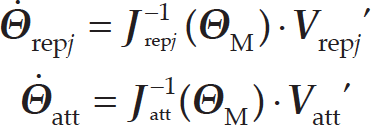
Θ˙₄ is the superimposed joint velocity vector of Θ˙₀, Θ˙₁, Θ˙₂ and Θ˙₃, which is inputted to the tool posture compensation module. The module output Θ˙₅, which is regarded as the final joint velocity signal, is sent to the joint actuators of the manipulator model.

When the collision-free path planning is finished, series data of discrete joint angle vector Θ versus time t are recorded and saved. The Cartesian space tool end path of the manipulator can be computed by the forward kinematics of Θ. This path is termed the “raw path”, and is illustrated in Figure 8. The trajectory generation system in the next sectin takes advantage of the raw path and generates joint space trajectory with continuous and smooth joint velocity.

4.2 Joint space trajectory generation system

In Figure 8, S and E are the predefined starting point and end point of the manipulator tool end, respectively. The tool end is expected to move along line SE where no obstacle exists. After obtaining the raw path from section 4.1, we divide it into three segment paths: SP ₁, P ₁ P ₂ and P ₂ E . It is important to note that V _att is active constantly in these three paths, while V _repj is only activated within path P ₁ P ₂.

The raw path adopts a relatively larger value of sampling interval t_s, while the generated path and corresponding joint space trajectory adopt smaller t_s values since the generated trajectory is used for joint motor actuation. Usually, the sampling interval t_s of generated trajectory should comply with the sampling interval set-up of the motion control card.

Figure 8.

Collision-free path planning and generation

4.2.1 Step one: Cartesian space cubic spline interpolation of pathP1P2

Path P ₁ P ₂ of the raw path is not smooth, such that the corresponding joint space trajectory is not smooth either, which will result in oscillation of manipulator movement. Therefore, Θ cannot be used for joint actuation directly. For this reason, cubic spline interpolation is adopted in order to ensure a continuous and smooth Cartesian path, while the tool end is guaranteed to pass through all the safe nodes at corresponding time moments.

The position coordinates X _s, Y _s and Z _s of all the safe nodes with corresponding time moment T _s are selected and outputted from the recorded data of raw-path data. Based on these data, cubic spline interpolation of safe nodes is done by the Matlab command “spline” with time variable of interpolation T _g = [T₁:t_s:T₂], which indicates the starting time moment T₁ and end time moment T₂ with sampling interval t_s=0.2 s. The command form of cubic spline interpolation is shown in Eq. (12). Finally, a series of continuous and smooth tool end position coordinates – X _g, Y _g and Z _g – of generated path P ₁ P ₂ with sampling interval t_s are obtained, as shown in Figure 8. The joint space trajectory due to tool end position coordinates X _g, Y _g and Z _g can be generated by inverse kinematics.

\begin{array}{l} X_{g} = spline (T_{s}, X_{s}, T_{g}); \\ Y_{g} = spline (T_{s}, Y_{s}, T_{g}); \\ Z_{g} = spline (T_{s}, Z_{s}, T_{g}); \end{array}

(12)

4.2.2 Step two: Joint space cubic polynomial interpolation of pathSP1, P1E

Step 1 produces a continuous and smooth Cartesian space path P ₁ P ₂ by cubic spline interpolation with corresponding joint space trajectory generated by inverse kinematics. However, it is important to note that the generated joint space velocities at points P ₁ and P ₂ are not zero. Consequently, in order to ensure the continuity and smoothness of joint space velocity within paths SP ₁ and P ₂ E , we deploy joint space cubic polynomial interpolation for these two paths. The joint angles at points S, P ₁, P ₂ and E can be acquired by inverse kinematics, while the joint velocities at points P ₁ and P ₂ can be computed by differential operation of joint angles at these points. Moreover, the joint space velocities at starting point S and end point E are both assumed to be zero. We will not detail the process of joint space cubic polynomial interpolation here, but will give the results in section 6.2.

5. Detour velocity

As mentioned in section 1, the potential field-based method has a drawback in that path planning may be trapped in local minimal; therefore, we deploy detour velocity and update the virtual repulsive velocity function in Eq. (7) to escape local minimal in a 3D environment.

Vector of detour force/velocity in a 2D environment can be calculated by equation P _j M _j / || P _j M _j ║90°, which is simple. Vector of detour force/velocity in a 3D environment can be multi-solution, as there are infinite vectors perpendicular to the repulsive velocity vector P _j M _j. In order to figure out appropriate directions of detour velocity, a simple and direct approach is introduced based on the three geometry primitives of SSV bounding boxes. This approach aims to specify the directional vector O _B O _A for each SSV bounding box, as illustrated in Figure 9; the vector of the detour velocity is then calculated by the vector cross-product.

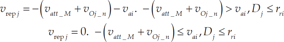
In Figure 10, M is the closest point on the manipulator, O _B O _A is the directional vector of an SSV bounding box, and M ′ is the projective point of M on line O _B O _A. After point M ′ is obtained, the vector of detour velocity can be computed by the cross-product of vectors M ′ M and O _BO_A.

Finally, the detour velocity is added into the virtual repulsive velocity function in Eq. (7) to produce the updated repulsive velocity function Eq. (13).

\begin{array}{l} V_{rep j} = v_{rep j} \cdot (O M / ‖ O M ‖ \pm k_{dv} \cdot {\hat{U}}_{dv}), k_{dv} > 0 \\ {\hat{U}}_{dv} = M' M \times O_{A} O_{B} / ‖ M' M \times O_{A} O_{B} ‖ \end{array}

(13)

Figure 9.

Specification of directional vector O _B O _A for SSV bounding boxes

Figure 10.

Determination of the vector of detour velocity in 3D environment

In Eq. (13), k_dv is the coefficient of detour velocity, which determines the magnitude of detour velocity. The greater the value of k_dv, the faster the manipulator detours around the obstacle, which results in shorter total task time and time-optimized path. However, increase in k_dv is constrained by joint angle, velocity and acceleration limits. Besides the joint space limits, we define a criterion to acquire a time-efficient path, that is, k_dv stops increasing when the total task time T decreases to the predefined task time T_d where no obstacle exists. These limits and this criterion should be complied when the time-efficient collision-free path is generated through increasing k_dv. In addition, since there are two directional vectors of M ′ M × O _B O _A, two standards are established for the choice of the unique directional vector. On the one hand, if one of the directional vectors traps in local minimal, then the other is chosen. On the other hand, the vector with shorter total task time is selected if no local minimal occurs for either directional vector.

6. Simulations, results and discussions

Three simulations are executed to verify our proposed virtual velocity algorithm with established offline collision-free path-planning and trajectory-generating systems. Simulation 1 verifies the established offline collision-free path-planning and trajectory-generating systems, introduced in section 4, and the evaluation of the effect of detour velocity presented in section 5. We compare our method with the other three virtual velocity-based methods in simulations 2 and 3. Discussions are also provided at the end of each simulation.

6.1 Conditions and setups of simulations

The robotic manipulator model, bounding box model, link parameters, joint angle and velocity limits have already been introduced in section 2. The establishment of the manipulator kinematics model, motion control and simulation are done by Solidworks-Simulink software, based on [39]. In consideration of simulation speed and the convenience of drawing, sampling interval t_s of raw path is set to 0.4 s and t_s of generated path and trajectory is set to 0.2 s.

Figure 11.

Scenario of a manipulator avoiding a moving obstacle

The scenario in simulations 1 and 2 is the same as that illustrated in Figure 11, which shows the collision avoidance between a six-DoF manipulator and a moving obstacle, represented by a LSS bounding box.

The origin of the manipulator (M) base coordinate system { R _m} is (0,0,0), and the starting point and end point of manipulator tool end are S (1700,1000,-400) and E (0,1000,-400), respectively. The initial position coordinates of the two vertices of the obstacle represented by an LSS bounding box are O _A (850,1000,900) and O _B (850,1000,-600) with bounding box radius r_Oj = 150 mm. T_d = 20 s is the desired total task time where no obstacle exists, while T is the actual total task time. The magnitude of obstacle moving velocity || V _Oj || = 13 mm/s for simulation 1; || V _Oj || = 13 mm/s and 20 mm/s for simulation 2. The virtual attractive velocity vector of manipulator tool end V _att is computed by Eq. (1), ω_att = (0,0,0), and the magnitude v_att of V _att can be computed by v_att = || SE || /T_d = 1700/20=85 mm/s. Meanwhile, virtual repulsive velocity vector V _repj without detour velocity is computed by Eq. (7), while V _repj with detour velocity is computed by Eq. (13) with safety radius of active region D_s = 80 mm, ω_repj = (0,0,0).

Simulation 3 is collision avoidance between two six-DoF manipulators. A dual-manipulator model is established with base coordinate system { R _m} = (0, 0, 0) of manipulator M. { R _m} is also the world coordinate system, which is shown in Figure 12. The origin of { R _s} is (1700,1650,0). The starting point and end point of tool end for manipulators M and S are S _m (1700, 1000, −400), E _m (0, 1000, −400) and S _s (50, 750, −400), E _s (1000, 0, −400), respectively.

T_d=20 s, while T is the actual total task time, which indicates the time length when both manipulators reach their respective destinations. V _att is computed by Eq. (1) and V _repj is computed by Eq. (7) and Eq. (13). v_att is still computed by v_att = || SE || /T_d Values for manipulators M and S are 85 mm/s and 60.5 mm/s, respectively. Safety radius of active region is D_s=80 mm for both manipulators.

Figure 12.

Scenario of collision avoidance between two manipulators

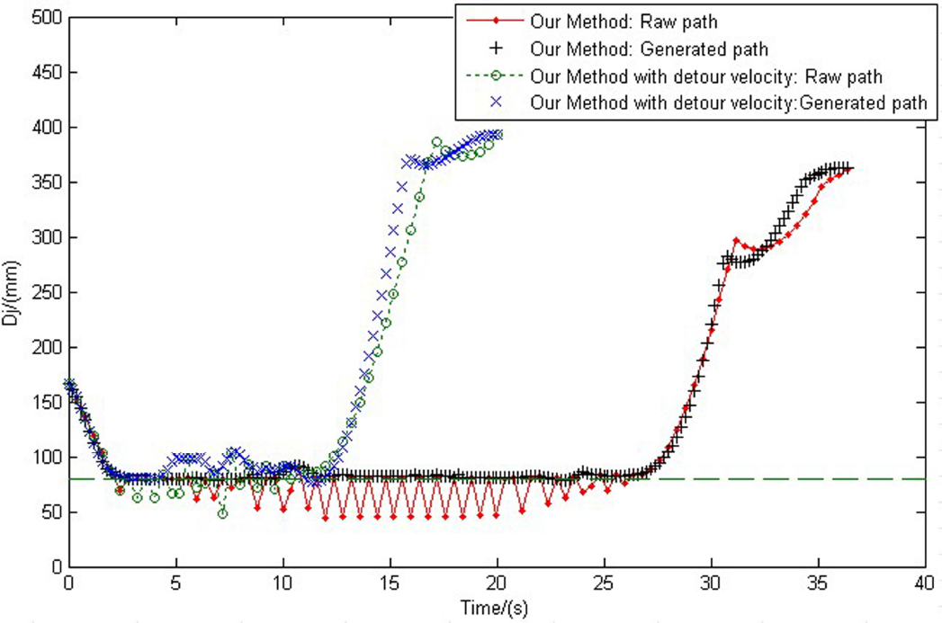
6.2 Simulation 1: Evaluation of proposed algorithm and system

The results of collision-free path planning and trajectory generation are illustrated in Figures 13–16. The total task time of path planning with detour velocity is reduced from 36.4 s to the expected optimal time 20 s when k_dv is increased to 1.6.

Figure 13 shows the generated manipulator tool end paths in Cartesian space. Graphically, path P ₁ P ₂, generated by Cartesian space cubic spline interpolation, and paths SP ₁ and P ₂ E , generated by joint space cubic polynomial interpolation, are all continuous and smooth even at the conjunction point of P ₁ and P ₂. The length of the path with detour velocity is shorter compared with the path without detour velocity.

Figure 13.

Results of collision-free path planning

Figure 14.

Generated joint space velocity with detour velocity

Figure 14 shows that the corresponding joint space velocity of path P ₁ P ₂, generated by Cartesian space cubic spline interpolation, is continuous and smooth. Moreover, joint space cubic polynomial interpolation of paths SP ₁ and P ₂ E can produce smooth joint velocity transition at the conjunction point of P ₁ and P ₂.

Figure 15 shows that the Cartesian space velocity of the whole generated path from starting point S to end point E is continuous and smooth within the whole task time. The addition of detour velocity can greatly shorten the total task time but may result in increase and fluctuation of Cartesian space velocity, especially within path P ₁ P ₂ since V_repj and detour velocity are only valid within this path. However, the Cartesian space velocity of the whole generated path is still continuous and smooth.

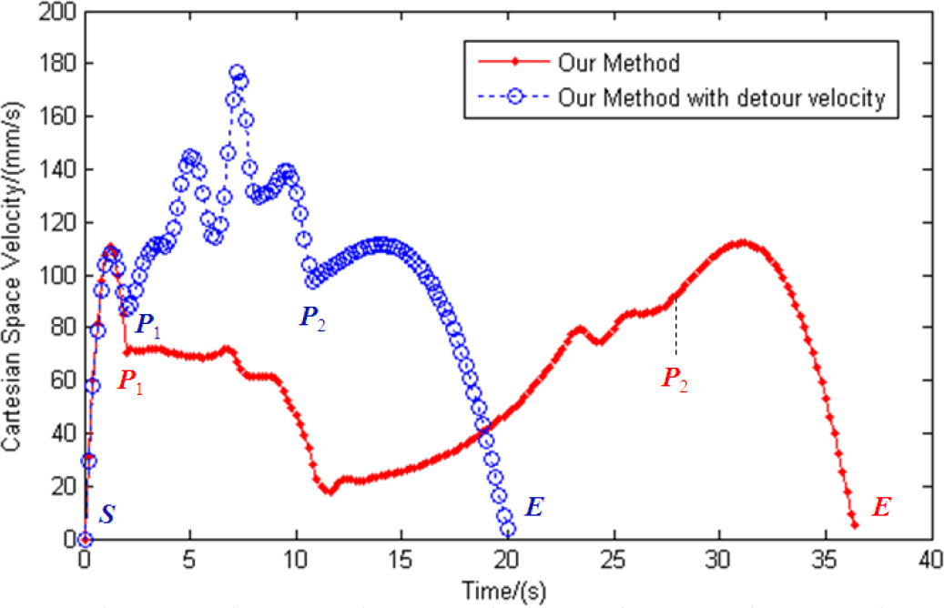
Figure 16 shows that employing V _repj without detour velocity can maintain the minimum distance D_j between a manipulator and a moving obstacle at the expected value D_s, which can satisfy the safety requirements in manufacturing applications. Meanwhile, the addition of detour velocity may result in fluctuation in the minimum distance curve but can still ensure D_j≥D_s during the movement.

Figure 15.

Cartesian space velocity curves of generated paths

Figure 16.

Curve of minimum distance Dj

In summary, the joint space trajectory generated by steps 1 and 2 in section 4.2 can ensure the continuity and smoothness of both joint space velocity and Cartesian space velocity. Therefore, the joint space trajectory generated by our proposed trajectory-generating system can be directly sent to the joint servomotors for motion control. Moreover, the addition of detour velocity can greatly shorten the total task time by adjusting and increasing the coefficient of detour velocity k_dv. Finally, the safety requirement of D_j≥D_s and the continuity and smoothness of joint space velocity during the movement can be all fulfilled.

6.3 Simulation 2: Methods comparison of collision avoidance between a manipulator and a moving obstacle

In this simulation we compare our method with the other three virtual velocity-based methods. Since the success of collision-free path planning mainly depends on the repulsive velocity, we use the same attractive velocity function Eq. (1) but different repulsive velocity functions for each method. The vector of repulsive velocity V _repj of our method is computed by Eqs. (7,13). The repulsive velocity functions of Eqs. (14–17) of V _repj for the other three methods are explained below. V _repj can be computed by V _repj=v_repj* P _j M _j /‖ P _j M _j‖, the same as in Eq. (7).

Repulsive velocity function 1 [29]: v_ai is the maximum allowed approaching velocity and Eq. (14) is the function of v_ai. The variables in Eq. (14) refer to [29]; we assume ${\hat{c}}_{i}^{T} V_{ip i} = 0$ , r_ri=1.5*D_s, r_ei= D_s, d_pi=D_j and adjust v_halfi to obtain an appropriate curve of v_ai.

v_{att_M}+v_{Oj_n} is the approaching velocity between the manipulator and the moving obstacle along the direction of minimum distance D_j, which is explained in section 3. The calculation of v_repj is according to Eq. (15).

v_{a i} = {\hat{c}}_{i}^{T} V_{ip i} + (v_{half i} / \ln (0.5)) \cdot \ln ((r_{r i} - d_{p i}) / (r_{r i} - r_{e i})) D_{j} \leq r_{r i} .

(14)

\begin{matrix} v_{rep j} = - (v_{a t t_M} + v_{O j_n}) - v_{a i} . - (v_{a t t_M} + v_{O j_n}) > v_{a i}, D_{j} \leq r_{r i} \\ v_{rep j} = 0. - (v_{a t t_M} + v_{O j_n}) \leq v_{a i}, D_{j} \leq r_{r i} \end{matrix}

(15)

Repulsive velocity function 2 [23] is according to Eq. (16): K_oj is the repulsive coefficient.

\begin{matrix} v_{rep j} = 0. D_{j} > D_{s} \\ v_{rep j} = K_{o j} (D_{j} / {| D_{j} |}^{r}), r > 1. 0 < D_{j} \leq D_{s} \\ v_{rep j} = + \infty . D_{j} < 0 \end{matrix}

(16)

Repulsive velocity function 3 [25] is according to Eq. (17): β is the repulsive coefficient.

\begin{matrix} v_{rep j} = 0. D_{j} > D_{s} \\ v_{rep j} = β (D_{s} - D_{j}), β > 0. 0 < D_{j} \leq D_{s} \\ v_{rep j} = + \infty . D_{j} < 0 \end{matrix}

(17)

Two simulations are demonstrated due to normal situation and situation of trapping in local minimal. The results of collision-free path planning for four velocity-based methods are given.

6.3.1 Normal situation

This simulation compares the performance of four virtual velocity-based methods in a normal situation. The results of collision-free path planning for the four methods are illustrated in Figure 17 and Table 2.

The adjustment of the parameters of methods 1, 2 and 3 is made on the basis of two criteria. On the one hand, the parameters should be large enough to “push” the manipulator away outside the active region D_s if the minimum distance D_j is less than D_s in consideration of safety requirements. On the other hand, the adjustment of parameters aims at obtaining an optimized path with shortest total task time.

Figure 17.

Comparison of four methods in normal situation

Figure 17 shows the manipulator tool end paths of the four methods in Cartesian space. The advantage of our method without detour velocity is not obvious compared with the other three methods. However, addition of detour velocity helps the manipulator to detour the moving obstacle much faster with the shortest length of path. This situation can also be observed from the total task time in Table 2.

Table 2.

Comparison of four methods on total task time

Repulsive velocity algorithm	Parameters	Total task time (s)
Method1 [29]	v_halfi = 110	39.6
Method 2 [23]	K_Oj=7400, r=2	42.4
Method 3 [25]	β=6	51.6
Our method (k_r=1.2)	k_dv = 0	36.4
Our method (k_r=1.2)	k_dv = 1.6	20

6.3.2 Situation of trapping in local minimal

The simulation condition of this section is the same as in section 6.3.1, except that the moving speed || V _Oj || of the obstacle is increased to 20 mm/s. The results of collision-free path planning for the four methods are illustrated in Figure 18.

Our method with detour velocity successfully reaches the goal and the total task time is reduced to 20 s when k_dv = 1.7 so that time-efficient path is obtained. The other three methods, along with our method without detour velocity, fail to reach the end point E .

In a word, the calculation for directional vector of detour velocity proposed in section 5 is valid and effective. The updated repulsive velocity function with detour velocity Eq. (13) is a simple and fast way of escaping local minimal in a 3D environment.

Figure 18.

Comparison of four methods where local minimal exists

6.4 Simulation 3: Methods comparison of collision avoidance between two manipulators

In section 6.3, only one manipulator is able to avoid the moving obstacle. However, in this section, both of the two manipulators are able to avoid each other. Applying virtual repulsive velocity function from Eq. (7) and Eq. (13) directly on both manipulators may result in a situation where D_j is approximately equal to twice D_s, since our method assumes that the moving obstacle is unable to avoid the manipulator. To address this issue, both of the manipulators apply 0.6* V _repj, which can effectively maintain D_j at D_s, ω_repj= (0,0,0).

The results of collision-free path planning for four methods are illustrated in Figure 19 and Table 3. Our method with detour velocity outperforms the other three methods at total task time. The corresponding joint space velocities for both manipulators applied with detour velocity in our method are continuous and smooth, but these are not presented due to page limitation.

Figure 19.

Generated collision-free paths of two manipulators

In addition, in Table 3 the total task time of time-efficient path T is equal to 21.2 s but not the expected time T_d = 20 s. The optimal total task time fails to reach 20 s because increasing k_dv can no longer reduce the total task time. This is because detour velocity is only valid within path P ₁ P ₂ in Figure 19. It reaches the limit when k_dv = 3. The time of paths SP ₁ and P ₂ E is determined by predefined attractive velocity V _att. This means that when the limit of detour velocity is reached but the optimal total task time is not yet obtained, we need to increase the magnitude of V _att to further reduce the total task time.

Table 3.

Comparison of four methods on total task time of two manipulators collision avoidance

Repulsive velocity algorithm	Parameters	Total task time (s)
Method 1 [29]	v_halfi = 25	34
Method 2 [23]	K_Oj=6500, r = 2	34.4
Method 3 [25]	β = 6.5	33.2
Our method (k_r = 12)	k_dv = 0	35.2
	k_dv = 1.5	23.6
	k_dv = 3	21.2

7. Conclusion

The proposed algorithm with established offline collision-free path-planning and trajectory-generating systems can produce time-efficient trajectory for industrial manipulator arms with continuous and smooth joint space velocity and Cartesian space velocity. The safety requirements of collision avoidance with moving obstacles and the manufacturing requirements of smooth movement in fixed tact time can be both fulfilled within a controlled industrial environment. Future research should focus on the collision avoidance of more complex obstacles and multiple moving obstacles.

Footnotes

8.

Project funded by China Postdoctoral Science Foundation (2014M562169).

References

Park

S.H.

Lee

B.H.

(2006) Analysis of robot collision characteristics using the concept of the collision map, Robotica, Vol. 24, No. 3, 2006, pp. 295–303.

Sukhan

Moradi

Kardaras

Sung-Kwon

(1997) Geometric collision detection and potential field based time delay planning for dual arm systems, 1997 IEEE International Conference on Robotics and Automation, pp. 882–887,1997.

Jianing

Nagase

Kimura

Aiyama

(2011) Collision avoidance of two manipulators using RT-Middleware, 2011 IEEE/SICE International Symposium on System Integration (SII), pp. 1031–1036, 2011.

Afaghani

A.Y.

Aiyama

(2013) On-line collision avoidance between two robot manipulators using collision map and simple escaping method, 2013 IEEE/SICE International Symposium on System Integration (SII), pp. 105–110, 2013.

Afaghani

A.Y.

Aiyama

(2014) Advanced-collision-map-based on-line collision and deadlock avoidance between two robot manipulators with PTP commands, 2014 IEEE International Conference on Automation Science and Engineering (CASE), pp. 1244–1251, 2014.

Medina

Taitz

Moshe

B.B.

Shvalb

(2013) C-Space Compression for Robots Motion Planning Int. J. Adv. Robot. Syst, Vol.10, No.6, 2013, Available from: http://www.intechopen.com/iournals/international_journal_of_advanced_robotic_systems/c-space-compression-for-robots-motion-planning. Accessed on 26 Mar 2014.

Ramirez-Gordillo

Merchan-Cruz

E.A.

Lugo-Gonzalez

. (2008) The Laplacian Artificial Potential Field (LAPF) for the Path Planning of Robotic Manipulators, 2008 Electronics, Robotics and Automotive Mechanics Conference (CERMA '08), pp. 508–513, 2008.

Rana

A.S.

Zalzala

A.M.S.

(1997) A neural networks based collision detection engine for multi-arm robotic systems, Fifth International Conference on Artificial Neural Networks, pp. 140–145, 1997.

Wang

(2011) Collision avoidance planning of manipulator based on C-space layered search arithmetic, 2011 International Conference on Electronic and Mechanical Engineering and Information Technology (EMEIT), pp. 3258–3262, 2011.

10.

Ralli

Hirzinger

(1994) Fast path planning for robot manipulators using numerical potential fields in the configuration space, in: Intelligent Robots and Systems (IROS), Proceedings of 1994 IEEE/RSJ/GI International Conference on Advanced Robotic Systems and the Real World, pp. 1922–1929, 1994.

11.

Mediavilla

Fraile

J.C.

Galindo

I.J.

Gonzalez

M.T.

(2003) Selection of strategies for collision-free motion in multi-manipulator systems, J. Intell. Robot. Syst., Vol. 38, No. 1, 2003, pp. 85–104.

12.

Khatib

(1985) Real-time obstacle avoidance for manipulators and mobile robots, Proceedings of 1985 IEEE International Conference on Robotics and Automation, pp. 500–505, 1985.

13.

Masoud

S.A.

Masoud

AA.

(2000) Constrained motion control using vector potential fields, IEEE Transactions on Systems, Man and Cybernetics, Part A: Systems and Humans, Vol. 30, No. 3, 2000, pp. 251–272.

14.

Khatib

Yokoi

Brock

Chan

g Casal

(1999) Robots in human environments: Basic autonomous capabilities, Int. J. Robot. Res., Vol. 18, No. 7, 1999, pp. 684–696.

15.

Babinec

Duchoň

Dekan

Pásztó

Kelemen

(2014) VFH/astTDT (VFH/ast with Time Dependent Tree): A new laser rangefinder based obstacle avoidance method designed for environment with non-static obstacles, Robotics and Autonomous Systems, Vol. 62, No. 8, 2014, pp. 1098–1115.

16.

Chuang

J.H.

Lin

C.C.

Chou

T.H.

(2006) An Alternate Priority Planning Algorithm for Dual-Arm Systems, 2006 IEEE International Symposium on Industrial Electronics, pp. 3084–3089, 2006.

17.

Byrne

Naeem

Ferguson

(2013) An intelligent configuration-sampling based local motion planner for robotic manipulators, 2013 Ninth Workshop on Robot Motion and Control (RoMo-Co), pp. 147–153, 2013.

18.

Braun

B.M.

Starr

Wood

J.E.

Lumia

(2004) A framework for implementing cooperative motion on industrial controllers, IEEE Transactions on Robotics and Automation, Vol. 20, No. 3, 2004, pp. 583–589.

19.

Bayro-Corrochano

Carbajal-Espinosa

Loukianov

(2010) Applications of potential fields and conformal geometric algebra for humanoid manipulation maneuvering 2010IEEE/RSJ International Conference on Intelligent Robots and Systems (IROS), pp.1378–1383, 2010.

20.

Carbajal-Espinosa

Loukianov

Bayro-Corrochano

(2010) Obstacle avoidance for a humanoid arm using conformal geometric algebra, 2010 Tenth IEEE-RAS International Conference on Humanoid Robots (Humanoids), pp. 524–529, 2010.

21.

Iossifidis

Schoner

(2006) Dynamical Systems Approach for the Autonomous Avoidance of Obstacles and Joint-limits for a Redundant Robot Arm, 2006 IEEE/RSJ International Conference on Intelligent Robots and Systems, pp. 580–585, 2006.

22.

Matveev

A.S.

Wang

Savkin

A.V.

(2012) Real-time navigation of mobile robots in problems of border patrolling and avoiding collisions with moving and deforming obstacles, Robotics and Autonomous Systems, Vol. 60. No. 6, 2012, pp. 769–788.

23.

Kitts

C.A.

Stanhouse

Chindaphorn

(2009) Cluster space collision avoidance for mobile two-robot systems, 2009 IEEE/RSJ International Conference on Intelligent Robots and Systems (IROS), pp. 1941–1948, 2009.

24.

Savkin

A.V.

Wang

(2014) Seeking a path through the crowd: Robot navigation in unknown dynamic environments with moving obstacles based on an integrated environment representation, Robotics and Autonomous Systems, Vol. 62, No. 10, 2014, pp. 1568–1580.

25.

Haghshenas Jaryani

(2007) An effective manipulator trajectory planning with obstacles using virtual potential field method, 2007 IEEE International Conference on Systems, Man and Cybernetics (ISIC), pp. 1573–1578, 2007.

26.

Ikeda

Tanaka

Zhang

T.X.

Minami

Mae

(2006) On-line Optimization of Avoidance Ability for Redundant Manipulator, 2006 IEEE/RSJ International Conference on Intelligent Robots and Systems, pp. 592–597, 2006.

27.

Daachi

Madani

Benallegue

(2012) Adaptive neural controller for redundant robot manipulators and collision avoidance with mobile obstacles, Neurocomputing, Vol. 79, 2012, pp. 50–60.

28.

Luo

R.C.

M.C.

Chung

Y.T.

Chatila

(2014) Repulsive reaction vector generator for whole-arm collision avoidance of 7-DoF redundant robot manipulator, 2014 IEEE/ASME International Conference on Advanced Intelligent Mechatronics (AIM), pp. 1036–1041, 2014.

29.

Bosscher

Hedman

(2011) Real-time collision avoidance algorithm for robotic manipulators, Ind. Robot., Vol. 38, No. 2, 2011, pp. 186–197.

30.

P.W.

Lin

Y.C.

Wang

CM.

L.C.

(2013) Grasping the object with collision avoidance of wheeled mobile manipulator in dynamic environments, 2013 IEEE/RSJ International Conference on Intelligent Robots and Systems (IROS), pp. 5300–5305, 2013.

31.

Zeng

L.Q.

Bone

G.M.

(2013) Mobile Robot Collision Avoidance in Human Environments, Int. J. Adv. Robot. Syst, Vol. 10, 2013, Available from: http://www.intechopen.com/journals/international_journal_of_advanced_robotic_systems/mobile-robot-collision-avoidance-in-human-environments. Accessed on 26 Mar 2014.

32.

Borenstein

Koren

(1989) Real-time obstacle avoidance for fast mobile robots, IEEE Transactions on Systems, Man and Cybernetics, Vol. 19, No. 5, 1989, pp. 1179–1187.

33.

Park

M.G.

Jeon

J.H.

Lee

M.C.

(2001) Obstacle avoidance for mobile robots using artificial potential field approach with simulated annealing, Proceedings of 2001 IEEE International Symposium on Industrial Electronics (ISIE), pp. 1530–1535, 2001.

34.

S.S.

Cui

Y.J.

(2000) New potential functions for mobile robot path planning, IEEE Transactions on Robotics and Automation, Vol. 16, No. 5, 2000, pp. 615–620.

35.

Zeng

L.Q

Bone

G.M.

(2010) Collision avoidance for nonholonomic mobile robots among unpredictable dynamic obstacles including humans, 2010 IEEE Conference on Automation Science and Engineering (CASE), pp. 940–947, 2010.

36.

Masoud

AA.

(2007) Decentralized Self-Organizing Potential Field-Based Control for Individually Motivated Mobile Agents in a Cluttered Environment: A Vector-Harmonic Potential Field Approach, IEEE Transactions on Systems, Man and Cybernetics, Part A: Systems and Humans, Vol. 37, No. 3, 2007, pp. 372–390.

37.

Larsen

Gottschalk

Lin

M.C.

Manocha

(1999) Fast proximity queries with swept sphere volumes, Tech. Report TR99-018. Department of Computer Science, Univ. of North Carolina (1999). Available from: http://gamma.cs.unc.edu/SSV/ssv.pdf. Accessed on 26 Mar 2014.

38.

Larsen

Gottschalk

Lin

M.C.

Manocha

(2000) Fast distance queries with rectangular swept sphere volumes, Proceedings of 2000 IEEE International Conference on Robotics and Automation (ICRA), pp. 3719–3726, 2000.

39.

Zhang

Ouyang

(2012) Offline motion planning and simulation of two-robot welding coordination, Front. Mech. Eng., Vol. 7, No. 1, 2012, pp.81–92.

Virtual Velocity Vector-Based Offline Collision-Free Path Planning of Industrial Robotic Manipulator

Abstract

Keywords

1. Introduction

2. Establishment of the bounding box model

3.1 Virtual velocity vectors

3.2.1 Attractive velocity function

4.1 Collision-free path-planning system in Cartesian space

5. Detour velocity

6.1 Conditions and setups of simulations

Footnotes

8.

References