
Abstract
Inventory represents an essential part of current assets, which are typically characterized by their transience.
This paper aims to outline a numerical solution of the inventory balance equation supplemented by an order-up-to replenishment policy for a case in which the problem is described by a differential equation with delayed argument. The results are demonstrated on a specific example and the behaviour of the model is presented using a computer simulation. The results are graphically shown in the Maple system. The solution makes use of the theory of functional differential equations, especially the part dealing with differential equations with delayed arguments.
1. Introduction
Increasing emphasis has been placed upon increasing labour productivity and the efficiency of managerial processes, as well as other activities within the company. Despite their undoubtedly positive function, inventories tend to be considered as a flaw in management work and the tendency is to reduce their amount to a minimum. As the state of the inventory is easily measurable and, thanks to the quality of current computer technology, the state of the inventory can be monitored across entire supply chains, inventory management has become a focus of specialists in mathematical methods in management.
One way of incorporating the dynamics of processes in a model is to describe it with differential equations. This paper deals with a numerical solution of the inventory balance equation supplemented by an order-up-to replenishment policy described by a differential equation with delayed argument. In the application section, the construction of a model is presented, including the possibilities of its solutions in a particular case. The behaviour of the model is demonstrated by means of computer simulation. Further, the equation of the model is solved by the modern theory of so-called ‘functional differential equations’, a specific part of which is a theory of linear differential equations with delayed arguments. The graphical presentation of the results uses the Maple system.
2. Literary review
Inventory represents the biggest investment in many companies. Lambert et al. [1] claim that inventory may account for more than 20% of total assets in production companies, while in business enterprises it may reach more than 50%. The increase in inventory has been caused by competition in the market over the past 20–25 years as companies have significantly expanded their assortment in an effort to meet the needs of various market segments. At the same time, customers have begun to demand very high availability of products.
A range of studies on inventory management in retail have been carried out, taking into account different aspects (e.g., see [2–5]).
Modern supply chains are often prone to instability in orders relating to the bullwhip effect (which is sometimes referred to as the ‘amplification effect’). The bullwhip effect refers to a problematic situation in a supply chain where, with a limited amount of information and locally limited decision-making, small variations in the end user's demand amplify upwards in the chain. Strictly speaking, starting with end users via shops and manufacturers and their suppliers, variability in demand in supply chains becomes increasingly higher.
The bullwhip effect was first mentioned by Forrester [6–7]. Other studies, e.g., [8–10], contain data on inventory volatility describing a similar effect. Similarly, Sterman in his BeerGame [11], designed for teaching the theory of inventory management, shows the same phenomenon. In the 1990s, Procter&Gamble experienced the bullwhip effect related to the production of and demand for Pampers nappies.
Countless studies have been carried out over the years and there is an extensive literature related to this issue [12–25]. The problem was examined using various possibilities provided, e.g., by probability theory [12–13], management theory [17–19], differential equations with delay [20], linear analysis of stability [21], the stochastic method of inventory management [22–23] and chaos theory [24]. Among other studies, Kim and Springer [25] can be mentioned, exploring two volatilities using systemic dynamics of a model which derives conditions of oscillation.
However, most of the studies aim to prove the existence of the bullwhip effect or to identify its causes, or else to determine possible counter-measures.
In his pioneering study, Forrester [6] examines the impact of demand on the function defining the state of inventory and the consequences of delay time in the process. The author also deduced an ordinary second-order differential equation with delay defining the examined model. Warburton [19] also employs differential equations with delay and takes advantage of the possibility of exponential approximation for a solution (Lambert's W function). The difficulty of this method lies in the fact that the resulting characteristic equation is transcendent and, as a result, the solution is conditioned by errors in the roots' approximation as well. The pitfalls of methods solving the mathematical models of the above-mentioned pioneer studies can be avoided by using solutions for differential equations and their systems with delay, which have been derived over recent decades. The method mentioned below is based on the fixed point theorem, more specifically on an operator affiliated with the problem. The method has a ‘global’ character (the solution is obtained by successive approximations simultaneously across the whole solution interval) and, from the numerical point of view, is stable.
3. An equation of inventory balance
A detailed derivation of an equation of inventory balance (which will be used in this chapter) can be found in the following publications [6, 19].
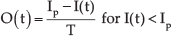
Let us assume that retailers attempt to minimize their inventory while maintaining it at a sufficient level to deal with standard fluctuations in demand. Thus, their objective is to fully satisfy the demand using inventory levels and allowing for stochastic effects. Demand for the supply of a certain amount of goods D(t) (the extent of demand per time unit) is always fulfilled. Failure to deliver is forbidden. The aim of inventory management is to maintain the current level of inventory I(t) around the required value Ip Inventory levels decline at the same rate at which demand D(t) is met and increases by the amount of replenished goods R(t). The balance of inventory is thus defined by equation (1):

We assume, in accordance with reality, that there is a certain time delay between an order and the supply of goods thereby caused, e.g., by the transportation time. It follows that the amount of replenished goods at time t equals the order made at the preceding time. Equation (2) can be applied to a situation in which the amount of replenished goods equals the amount of goods ordered at time t – τ:

As the inventory is gradually depleted based on demand, it is also replenished to in order to bring the inventory back towards the desired value. In paper [19] an equation of a replenishment policy is defined in which the size of an order is directly proportional to the shortage of inventory:
and:

Ip represents the required level of inventory. If the demand unexpectedly increases, the inventory is gradually replenished but, thanks to a facultative parameter T, the replenishment can be spread over a longer period. If delays in supplies are long, this might result in a significant increase in inventory, which is unwelcome [6]. Therefore, it is advisable to include equation (4) in the model, which adds constraints allowing for the suspension of any replenishment if its level exceeds the required value [12, 18–19].
4. Differential equations with a delay argument
Modelling phenomena which arise from economic reality and which are described by statistical data are possible thanks to methods based predominantly on mathematical disciplines, such as statistics, numerical methods, operational research, linear and dynamic programming, and optimization, etc. (e.g., see [26–30]). One way of giving a true picture of the dynamics of processes in a model is to describe a dynamic model using differential equations. If we utilize this possibility, we have to understand time as a continuous quantity, which allows us to exploit an elaborate mathematical setup of differential and integral calculus. The outcome is not an estimate of the parameters of a pre-defined function but rather is a function per se, whose shape gives evidence of the nature of the examined quantities.
Let us focus on special cases of functional differential equations, i.e., differential equations with a delayed argument and their solutions. As early as the 1950s, new mathematical models were being developed which could be used for a real description of various processes from practical life [31–34.]. This development went hand in hand with the development of ‘Carathéodory's theory’ of differential equations, specifically with the theory of functional differential equations.
The available literature dealing with the solvability of systems of differential equations with delayed arguments offers a range of results applicable when solving problems from economic practice. In their papers, the authors deal with conditions for the solvability of the given problems (i.e., existence and unambiguity of a solution), conditions for their correctness (i.e., a small change in initial conditions corresponds with a small change in the final solution), conditions for the non-negativity of a solution, and many others. A description of the method enabling the construction of a numerical solution can also be found there.
The general theory, which focuses on solutions for the above-stated problems and related problems, can be studied in [35–38]. An application problem based on solving systems of differential equations with delayed argument, including the description of a solution, can be found in, e.g., [39], and in the literature cited in it.
The construction of a solution for our problem was made using the Maple system. Maple is mathematical software, an advantage of which is the possibility of finding a solution in a symbolic manner.
In order to find a solution for our problem, numerical methods built in Maple are used which are designed to find solutions for ordinary differential equations as well as the above-mentioned modern theory of solving differential equations with a delayed argument.
5. Analysis of the solution of an equation using modern theory
Given the current familiarity with differential equations with a delayed or – more generally – deviated argument (or so-called ‘functional differential equations’), we have the possibility to apply the method of solving a significantly more general mathematical model, which may provide us with a wider range of results, including a comparison of the impact that various parameters might have.
Let us present a mathematical model defined at the beginning of the economic process on interval [0,T]:

We will have:

and:

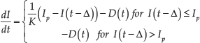
It is evident that equation (5) with condition (6) can be written down as:

Therefore:

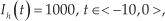
At the same time, a natural consequence of a continuous sequence of solutions I(t) from the interval [0, T] to the ‘historic’ function h (t) (t[-Δ, 0]) is an initial condition of solution I(t) of equation (3) in the following way:

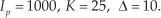
Moreover, it follows from (1–4) that Ip>0, Δ>0, K>0 are constants and that D(t) and h(t) are continuous functions.
Consequently, problems (5) and (6) are equivalent to problems (10) and (11) (see [38–39]), and the listed bibliography on fully general linear boundary value problems for functional differential equations gives evidence to the following:
The unambiguous solvability of problems (3), (4), (10) and (11).
The possibility of a solution using the method of successive approximations.
Under these conditions, problems (5) and (6) have one, and only, solution, and the solution is continuously differentiable on interval [0, T]. If functions D(t) and h(t) had jump discontinuities in corresponding intervals, the solution of tasks (5) and (6) would be continuous but would not have a derivative in the corresponding points.
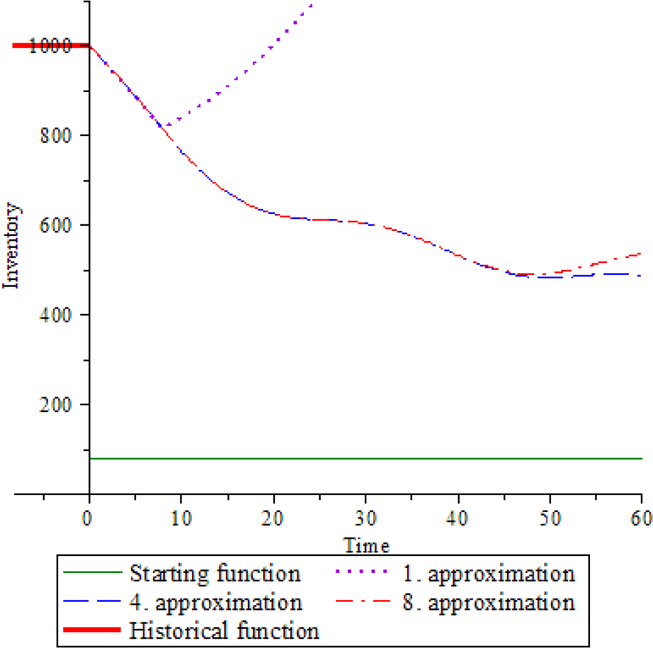
Analogically to the method utilized in the above-mentioned studies, we will use the method of successive approximations in order to find the solution for tasks (10) and (11):
We select, at random, function I0, which is continuous on interval [0,T], e.g., I0(t)=h(0), tε[0,T].
We successively calculate the nth approximation of the sought-for solution, n ε N, using additional problems.


In order to determine the accuracy of the approximation, we can, given the conditions of the problem, use an estimate:

From the correctness of problems (10) and (11) (the Cauchy problem for the linear scalar constant coefficient differential equation with constant delay and continuous non-homogeneous members), and from the continuity of the solutions for problems (12) and (13), it follows that progression {In(t)} converges evenly on interval [0, T] towards solution for problems (10) and (11); therefore, ε n → 0 for n → + ∞. The calculation itself, ε n , may be replaced by an estimate calculated in a ‘sufficiently’ large number of points of interval [0,T]. This procedure can be applied to constructing the nth approximation of a solution with the accuracy given in advance.
In order to explore more profoundly the features of our problem's solution, we will apply the existing results concerning the oscillatoricity of a solution for a first-order linear differential equation with constant delay. For example, it follows from [40] that each equation:

is oscillatory (i.e., it has infinitely many zero points) if:
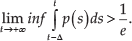
Therefore, the condition for the oscillatoricity of a solution of a homogeneous equation affiliated with (10) is:
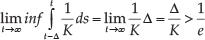
Consequently, the linearity of a problem means that the solution for our non-homogeneous problems (10) and (11), while meeting condition (17), will not be monotonous.
Approximation (source: Ourselves)
The model's behaviour in specific situations is comprehensively summarized in Tables 1 and 2:
The model's behaviour when conditions for oscillation are met (source: author's own solution)
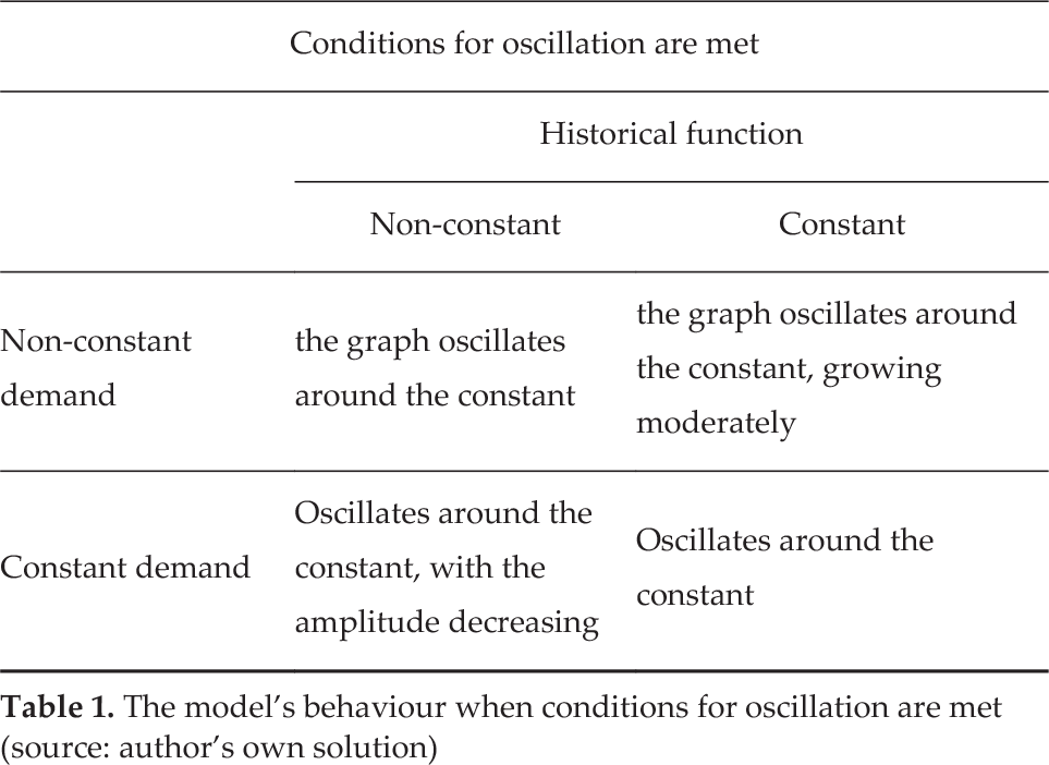
The model's behaviour when conditions for oscillation are met (source: author's own solution).

6. Illustrative examples


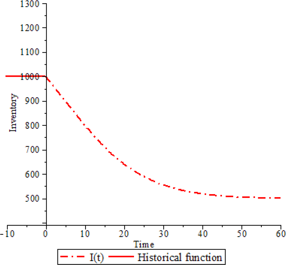
Even in this case, the condition of oscillatoricity was met and the calculated solution is shown in Fig. (2). It is evident that the value of inventory will indeed oscillate over time.


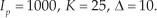
In this case, the condition of oscillatoricity was not met. The calculated solution is shown in Fig. (3) and it is apparently monotonous and falls towards a constant value.


In all four cases (2a, 2b, 2c, 2d), the model's parameters do not lead to an oscillatory solution. However, the non-constantness of functions Ih(t) and D(t) deforms the solution by moderate oscillation (Figs. 4–7). We can observe in 2d that a change in parameter Ip (a decrease) results in a change in the level at which inventory tends to level out over a longer period of time (in Fig. 2d it is a lower value than in Fig. 2c).

Oscillating solution (Source: ourselves)
Non-oscillating solution (source: ourselves)

Non-constant historical function, (source: ourselves)

Non-constant demand (source: ourselves)

Non-constant demand and non-constant historical function (source: ourselves)
I(0)≠ Ip (source: ourselves)
7. Conclusion
When modelling complex economic problems, we are often faced with the fact that the relations of particular quantities are variable in time. One way of incorporating the dynamics of processes in a model is to consider time as a continuous quantity and to describe dynamical models by means of differential equations. When specifying a model's structure, the dynamic character may be taken into account by incorporating the delayed impact of both exogenous and endogenous variables.
This paper presented a solution of the inventory balance equation supplemented by an order-up-to replenishment policy if it is presented by an ordinary differential equation with delayed argument. The equation is solved using the modern theory, and the impact of specific parameters of the model on its solution is analyzed.
We have also analysed the conditions for the oscillatoricity of solutions and situations in which the historic function and the demand function are not constant.
The theoretical results have been clarified by an illustrative example, which also provides a graphical representation of the specific results.
The model discussed in this paper could be expanded in the future. One option is the generalization of the model, which would allow us to work even with non-constant delay, etc.
Footnotes
8. Acknowledgements
This paper was supported by grant FP-S-13-2148 ‘The Application of ICT and Mathematical Methods in Business Management’ of the Internal Grant Agency at Brno University of Technology.