Improving the two-stage numerical integration in stability identification of oscillation with distributed delay

Abstract

The vibration of the engineering systems with distributed delay is governed by delay integro-differential equations. Two-stage numerical integration approach was recently proposed for stability identification of such oscillators. This work improves the approach by handling the distributed delay—that is, the first-stage numerical integration—with tensor-based higher order numerical integration rules. The second-stage numerical integration of the arising methods remains the trapezoidal rule as in the original method. It is shown that local discretization error is of order $\mathcal{O}(\mathrm{\Delta }t{)}^3$ irrespective of the order of the numerical integration rule used to handle the distributed delay. But $(\mathrm{\Delta }t{)}^3$ is less weighted when higher order numerical integration rules are used to handle the distributed delay, suggesting higher accuracy. Results from theoretical error analyses, various numerical rate of convergence analyses, and stability computations were combined to conclude that—from application point of view—it is not necessary to increase the first-stage numerical integration rule beyond the first order (trapezoidal rule) though the best results are expected at the second order (Simpson’s 1/3 rule).

Introduction

Oscillations with distributed delay are governed by delay integro-differential equations (DIDEs). DIDEs are applied in modeling biological and physical phenomena ¹ ; therefore, they have been viewed with growing importance by researchers. Baker and Ford ² applied a set of linear multistep methods mixed with quadrature rules to numerically solve Volterra DIDEs. A numerical scheme for reliably computing the stability-determining characteristic roots of DIDEs has been developed based on linear multistep method and a quadrature method based on Lagrange interpolation and a Gauss–Legendre quadrature rule. ³ Numerical methods based on backward differentiation formulae and repeated quadrature formulae for the solution of Volterra DIDEs were suggested by Zhang and Vandewalle. ⁴ Yeniçerioğlu ⁵ established several theorems on the behavior of solutions of scalar linear second-order-delay DIDEs. Like most of the afore-cited works, Huang ⁶ considered the preservation of the stability properties of DIDEs after some form of discretization based on linear multistep methods. Linear multistep quadrature rules were used by Wu and Gan ⁷ to find a numerical solution of singularly perturbed Volterra DIDEs. Rihan et al. ⁸ developed a method for numerical solution and for investigating the stability of Volterra DIDEs. They treated the differential part of Volterra DIDEs with the mono-implicit Runge–Kutta method and treated the integral part with the collocation method based on the Boole’s quadrature rule. Using Lyapunov’s functional approach, they discussed the stability properties of solutions of nonlinear Volterra DIDEs.

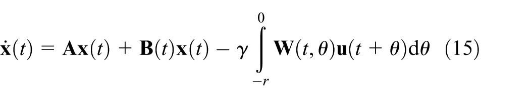
Beyond numerical stability and solution of DIDEs with known history at isolated parameter coordinates, engineering applications encounter periodic DIDEs with unknown history but requiring dynamical stability analysis for identification of the stability boundaries that delineate the parameter space into dynamically stable and unstable sub-domains so that smooth engineering operations can be selected systematically, even by the non-academic operators/users. An attempt in this direction by Rihan et al. ⁸ was limited to a scalar autonomous case which is amenable to pure analytical manipulation. The DIDEs modeling real engineering systems tend to be non-autonomous, therefore requiring more challenging identification protocol for the stability boundaries. In engineering, DIDEs have found applications in modeling regenerative vibrations^9,10 and wheel shimmy. ¹¹ The general form of DIDE, capturing the type studied here, is represented as follows ¹²

$$\stackrel{·}{\mathbf{x}}\left(t\right)=f(\mathbf{x}\left(t\right),\underset{-r}{\overset{0}{\int }}{\mathrm{d}}_{\theta }\mathbf{\eta }(t,\theta )\mathbf{x}(t+\theta ))$$

(1)

where $t>0,\mathbf{x}(t)\in {\mathbb{R}}^n,r\in {\mathbb{R}}_{+}$ is the duration of the distributed delay; $f:{\mathbb{R}}^n\times {\mathbb{R}}^n\to {\mathbb{R}}^n$ is a continuously differentiable function; $\mathbf{\eta }:\mathbb{R}\times \mathbb{R}\to {\mathbb{R}}^{n\times n}$ ; and $\mathbf{x}(t)=\mathbf{g}(t)$ for $t\in [-r,0]$ , where $\mathbf{g}(t)$ is called the history. The term containing the delay is the Stieltjes integral which has both discrete and distributed time delay

$$\underset{-r}{\overset{0}{\int }}{\mathrm{d}}_{\theta }\mathbf{\eta }(t,\theta )\mathbf{x}(t+\theta )=\sum _{j=1}^l{\mathbf{R}}_j\mathbf{x}(t-{\tau }_j)+\underset{-r}{\overset{0}{\int }}\mathbf{W}(t,\theta )\mathbf{x}(t+\theta )\mathrm{d}\theta$$

(2)

where ${\tau }_j\in {\mathbb{R}}_{+}$ are the discrete delays and $\mathbf{W}:\mathbb{R}\times \mathbb{R}\to {\mathbb{R}}^{n\times n}$ is the kernel function. The DIDEs studied here are the ones without discrete delays, and therefore given as follows

$$\stackrel{·}{\mathbf{x}}\left(t\right)=f(\mathbf{x}\left(t\right),\underset{-r}{\overset{0}{\int }}\mathbf{W}(t,\theta )\mathbf{x}(t+\theta )d\theta )$$

(3)

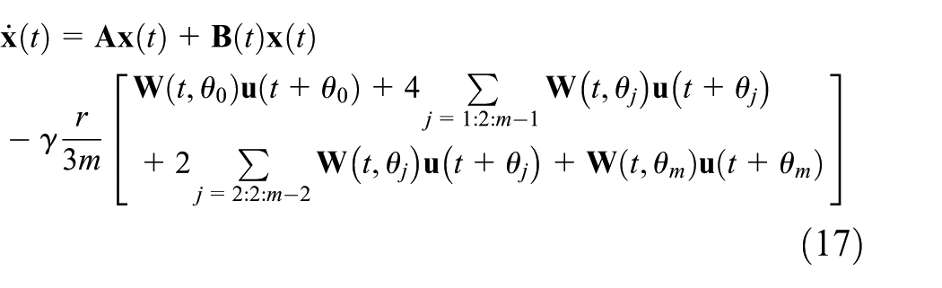
The stability boundaries of a class of non-autonomous DIDEs, as represented in equation (3), have been carried out with the semi-discretization method ¹² and the spectral finite element method. ¹³ Based on an accurate and time-saving full-discretization method, Ozoegwu ¹⁴ used two-stage numerical integration (NI) to identify the stability boundaries of the same class of DIDEs. The first-stage NI converted the distributed delay to a series of discrete delays, transforming equation (3) to a form without integral

$$\stackrel{·}{\mathbf{x}}\left(t\right)=f(\mathbf{x}\left(t\right),\left[\sum _{j=0}^m{C}_j\mathbf{W}(t,{\theta }_j)\mathbf{x}(t+{\theta }_j)\right])$$

(4)

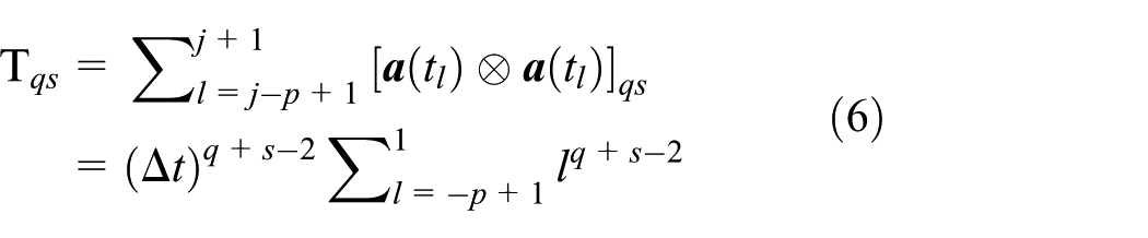
where $C_j$ are the coefficients that depend on the limits of integration, number of equal intervals m, and the order of NI rule. The second-stage NI was used to construct the monodromy matrix of the system. The second-stage NI is analogous to the application of NI methods in stability analysis of single-discrete delay models of milling process.^15–18 Ozoegwu ¹⁴ handled the distributed delay with trapezoidal rule. This work proposes to theoretically and numerically investigate the implications on accuracy and computational time of handling the distributed delay with higher order NI rules.

Tensor-based NI rules

Ozoegwu ¹⁴ used the trapezoidal rule to handle the distributed delay. This work proposes to consider the generalized higher order NI rules. In deriving the NI rules, the first step is discretizing the t-axis into m equal intervals $[t_j,t_{j+1}]$ where $j=0,1,2,\dots ,m-1$ and $\mathrm{\Delta }t=(t_m-t_0)/m=t_{j+1}-t_j$ . The second step is constructing m discrete areas $A_j$ which are bounded by $t=t_j$ , $t=t_{j+1}$ , the t-axis, and an integrand which in this case is a polynomial. The $A_j$ is then taken in multiple steps to generate higher order NI rules. The polynomial function $\mathit{f}(t)$ is formulated in a discrete interval as polynomial tensor

$$\mathit{f}\left(t\right)={\left[\mathit{a}\left(t\right)\right]}^T{\mathbf{T}}^{-1}\mathbf{Bv}={\left[\mathit{a}\left(t\right)\right]}^T\mathbf{Nv}$$

(5)

where $\mathit{a}(t)=\{\begin{array}{ccccc}1\hfill & t\hfill & t^2\hfill & \cdots \hfill & t^p\hfill \end{array}{\}}^T$ is the vector of polynomial basis, $\mathbf{T}$ and $\mathbf{B}$ are $(p+1)$ × $(p+1)$ numerical matrices, and $\mathbf{v}$ is a vector of discrete states. The elements of $\mathbf{T}$ are given as follows

$$\begin{array}{c}\multicolumn{1}{c}{{\mathrm{T}}_{\mathrm{qs}}=\sum _{l=j-p+1}^{j+1}{[\mathit{a}\left(t_l\right)\otimes \mathit{a}\left(t_l\right)]}_{\mathrm{qs}}}\\ \multicolumn{1}{c}{={\left(\mathrm{\Delta }t\right)}^{q+s-2}\sum _{l=-p+1}^1{l}^{q+s-2}}\end{array}$$

(6)

where ⊗ is the outer product operation. The elements of the matrix $\mathbf{B}$ and those of the vector $\mathbf{v}$ are given as follows

$${\mathrm{B}}_{\mathrm{qs}}=s_{j-p+s}^{q-1}={(s-p)}^{q-1}{\left(\mathrm{\Delta }t\right)}^{q-1}$$

(7)

$${\mathrm{v}}_q={\mathit{f}}_{j+q-p}$$

(8)

A pth-order NI rule becomes

$${\mathbf{A}}_j^{\mathrm{pth}}=\underset{t_{j-(p-1)}}{\overset{t_{j+1}}{\int }}\mathit{f}\left(t\right)\mathrm{dt}=\underset{(-p+1)\mathrm{\Delta }t}{\overset{\mathrm{\Delta }t}{\int }}\mathit{f}\left(t\right)\mathrm{dt}$$

(9)

In this work, the second-order NI rule (Simpson’s 1/3) and the third-order NI rule (Simpson’s 3/8) are considered. Substituting $p=2$ in the above equations gives the vector Simpson’s 1/3 rule as

$${\mathbf{A}}_j^{2\mathrm{nd}}=\frac{\mathrm{\Delta }t}{3}[{\mathit{f}}_{j-1}+4{\mathit{f}}_j+{\mathit{f}}_{j+1}]$$

(10)

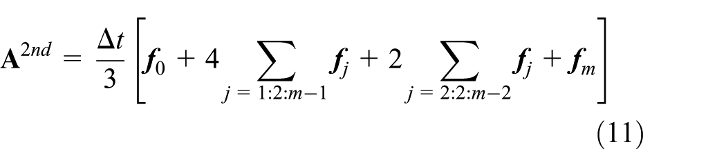
Considering all the ${\mathbf{A}}_j^{2\mathrm{nd}}$ , the composite Simpson’s 1/3 rule becomes

$${\mathbf{A}}^{2\mathrm{nd}}=\frac{\mathrm{\Delta }t}{3}[{\mathit{f}}_0+4\sum _{j=1:2:m-1}{\mathit{f}}_j+2\sum _{j=2:2:m-2}{\mathit{f}}_j+{\mathit{f}}_m]$$

(11)

Substituting $p=3$ in equation (9) and manipulating as appropriate gives the vector Simpson’s 3/8 rule as

$${\mathbf{A}}_j^{3\mathrm{rd}}=\frac{3\mathrm{\Delta }t}{8}[{\mathit{f}}_{j-2}+3{\mathit{f}}_{j-1}+3{\mathit{f}}_j+{\mathit{f}}_{j+1}]$$

(12)

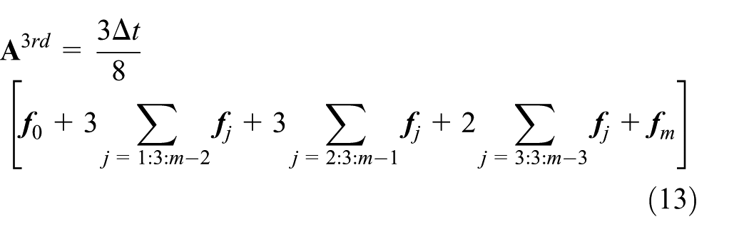
The composite Simpson’s 3/8 rule becomes

$${\mathit{A}}^{3rd}=\frac{3\mathrm{\Delta }t}{8}\left[{\mathit{f}}_0+3\sum _{j=1:3:m-2}{\mathit{f}}_j+3\sum _{j=2:3:m-1}{\mathit{f}}_j+2\sum _{j=3:3:m-3}{\mathit{f}}_j+{\mathit{f}}_m\right]$$

(13)

By substituting higher values of p in equation (9), higher order NI rules are generated and used, as long as that improves accuracy. But as later seen, there may not be any need to go beyond the third-order NI rule.

New two-stage NI methods

The non-autonomous DIDE studied in the literature,^12–14 and to be studied here for direct comparison, is the scalar second-order system

$$\stackrel{··}{x}\left(t\right)+\kappa \stackrel{·}{x}\left(t\right)+[\delta +ϵ\cos \left(\omega t\right)]x\left(t\right)=\gamma \underset{-r}{\overset{0}{\int }}\mathrm{w}(t,\theta )x(t+\theta )\mathrm{d}\theta$$

(14)

Making use of the substitutions $x_1(t)=x(t)$ and $x_2(t)=\stackrel{·}{x}(t)$ , the first-order form becomes

$$\stackrel{·}{\mathbf{x}}\left(t\right)=\mathbf{Ax}\left(t\right)+\mathbf{B}\left(t\right)\mathbf{x}\left(t\right)-\gamma \underset{-r}{\overset{0}{\int }}\mathbf{W}(t,\theta )\mathbf{u}(t+\theta )\mathrm{d}\theta$$

(15)

$$\mathbf{u}\left(t\right)=\mathbf{Dx}\left(t\right)$$

(16)

The matrix $\mathbf{A}=\left[\begin{array}{cc}0\hfill & 1\hfill \\ \multicolumn{1}{c}{-\delta }& -\kappa \hfill \end{array}\right]$ is the constant coefficient matrix that captures the transient response of the system dynamics, $\mathbf{B}(t)=\left[\begin{array}{cc}0\hfill & 0\hfill \\ \multicolumn{1}{c}{-ϵ\cos (\omega t)}& 0\hfill \end{array}\right]$ is the matrix valued function with period T that captures the forced component of the system dynamics, $\mathbf{x}(t)=\{\begin{array}{cc}x(t)\hfill & \stackrel{·}{x}(t)\hfill \end{array}{\}}^{\mathrm{T}}$ , $\mathbf{x}(t+\theta )=\{\begin{array}{cc}x(t+\theta )\hfill & \stackrel{·}{x}(t+\theta )\hfill \end{array}{\}}^{\mathrm{T}}$ , $\mathbf{W}(t,\theta )=\{\begin{array}{cc}0\hfill & -\mathrm{w}(t,\theta )\hfill \end{array}{\}}^{\mathrm{T}}$ , and $\mathbf{D}=\{\begin{array}{cc}1\hfill & 0\hfill \end{array}\}$ .

Method based on Simpson’s 1/3 rule

Applying equation (11) to the distributed delay of equation (15) gives

$$\begin{array}{c}\multicolumn{1}{c}{\stackrel{·}{\mathbf{x}}\left(t\right)=\mathbf{Ax}\left(t\right)+\mathbf{B}\left(t\right)\mathbf{x}\left(t\right)}\\ \multicolumn{1}{c}{-\gamma \frac{r}{3m}\left[\begin{array}{c}\mathbf{W}(t,{\theta }_0)\mathbf{u}(t+{\theta }_0)+4\sum _{j=1:2:m-1}\mathbf{W}(t,{\theta }_j)\mathbf{u}(t+{\theta }_j)\hfill \\ \multicolumn{1}{c}{+2\sum _{j=2:2:m-2}\mathbf{W}(t,{\theta }_j)\mathbf{u}(t+{\theta }_j)+\mathbf{W}(t,{\theta }_m)\mathbf{u}(t+{\theta }_m)}\end{array}\right]}\end{array}$$

(17)

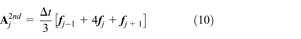
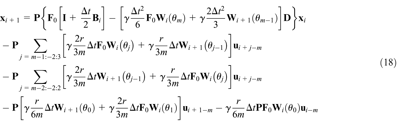
The distributed delay has been converted to a series of discrete delays. Equation (17) is discretized into k discrete intervals, $[t_i,t_{i+1}]$ , each of size $\mathrm{\Delta }t=t_{i+1}-t_i=T/k$ , where $t_i=i\mathrm{\Delta }t$ , $i=0,1,2,\dots ,(k-1)$ . Following the procedure in Ozoegwu, ¹⁴ equation (17) is solved as a linear ordinary differential equation (ODE) in each of the intervals $[t_i,t_{i+1}]$ using Duhamel’s integral and then handled with the trapezoidal rule to give the discrete transition

$$\begin{array}{c}\multicolumn{1}{c}{{\mathbf{x}}_{i+1}=\mathbf{P}\{{\mathbf{F}}_0[\mathbf{I}+\frac{\mathrm{\Delta }t}{2}{\mathbf{B}}_i]-[\gamma \frac{\mathrm{\Delta }{t}^2}{6}{\mathbf{F}}_0{\mathbf{W}}_i\left({\theta }_m\right)+\gamma \frac{2\mathrm{\Delta }{t}^2}{3}{\mathbf{W}}_{i+1}\left({\theta }_{m-1}\right)]\mathbf{D}\}{\mathbf{x}}_i}\\ \multicolumn{1}{c}{-\mathbf{P}\sum _{j=m-1:-2:3}[\gamma \frac{2r}{3m}\mathrm{\Delta }t{\mathbf{F}}_0{\mathbf{W}}_i\left({\theta }_j\right)+\gamma \frac{r}{3m}\mathrm{\Delta }t{\mathbf{W}}_{i+1}\left({\theta }_{j-1}\right)]{\mathbf{u}}_{i+j-m}}\\ \multicolumn{1}{c}{-\mathbf{P}\sum _{j=m-2:-2:2}[\gamma \frac{2r}{3m}\mathrm{\Delta }t{\mathbf{W}}_{i+1}\left({\theta }_{j-1}\right)+\gamma \frac{r}{3m}\mathrm{\Delta }t{\mathbf{F}}_0{\mathbf{W}}_i\left({\theta }_j\right)]{\mathbf{u}}_{i+j-m}}\\ \multicolumn{1}{c}{-\mathbf{P}[\gamma \frac{r}{6m}\mathrm{\Delta }t{\mathbf{W}}_{i+1}\left({\theta }_0\right)+\gamma \frac{2r}{3m}\mathrm{\Delta }t{\mathbf{F}}_0{\mathbf{W}}_i\left({\theta }_1\right)]{\mathbf{u}}_{i+1-m}-\gamma \frac{r}{6m}\mathrm{\Delta }t\mathbf{P}{\mathbf{F}}_0{\mathbf{W}}_i\left({\theta }_0\right){\mathbf{u}}_{i-m}}\end{array}$$

(18)

where

$${\mathbf{F}}_0={\mathrm{e}}^{\mathbf{A}\mathrm{\Delta }t}$$

(19)

$$\mathbf{P}={[\mathbf{I}-\frac{\mathrm{\Delta }t}{2}{\mathbf{B}}_{i+1}+\gamma \frac{\mathrm{\Delta }{t}^2}{6}{\mathbf{W}}_{i+1}\left({\theta }_m\right)\mathbf{D}]}^{-1}$$

(20)

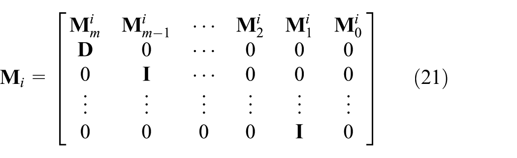
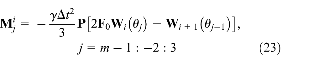
The $(m+n)$ -dimensional transition from state ${\mathbf{y}}_i$ to state ${\mathbf{y}}_{i+1}$ due to the action of a linear operator ${\mathbf{M}}_i$ is constructed from equation (18) as ${\mathbf{y}}_{i+1}={\mathbf{M}}_i{\mathbf{y}}_i$ such that ${\mathbf{y}}_{i+1}=\{\begin{array}{cccc}{\mathbf{x}}_{i+1}\hfill & {\mathbf{u}}_i\hfill & \cdots \hfill & {\mathbf{u}}_{i-m+1}\hfill \end{array}{\}}^T$ , ${\mathbf{y}}_i=\{\begin{array}{cccc}{\mathbf{x}}_i\hfill & {\mathbf{u}}_{i-1}\hfill & \cdots \hfill & {\mathbf{u}}_{i-m}\hfill \end{array}{\}}^T$ , and

$${\mathbf{M}}_i=\left[\begin{array}{cccccc}{\mathbf{M}}_m^i\hfill & {\mathbf{M}}_{m-1}^i\hfill & \cdots \hfill & {\mathbf{M}}_2^i\hfill & {\mathbf{M}}_1^i\hfill & {\mathbf{M}}_0^i\hfill \\ \multicolumn{1}{c}{\mathbf{D}}& 0\hfill & \cdots \hfill & 0\hfill & 0\hfill & 0\hfill \\ \multicolumn{1}{c}{0}& \mathbf{I}\hfill & \cdots \hfill & 0\hfill & 0\hfill & 0\hfill \\ \multicolumn{1}{c}{⋮}& ⋮\hfill & ⋮\hfill & ⋮\hfill & ⋮\hfill & ⋮\hfill \\ \multicolumn{1}{c}{0}& 0\hfill & 0\hfill & 0\hfill & \mathbf{I}\hfill & 0\hfill \end{array}\right]$$

(21)

where

$${\mathbf{M}}_m^i=\mathbf{P}\{{\mathbf{F}}_0[\mathbf{I}+\frac{\mathrm{\Delta }t}{2}{\mathbf{B}}_i]-[\gamma \frac{\mathrm{\Delta }{t}^2}{6}{\mathbf{F}}_0{\mathbf{W}}_i\left({\theta }_m\right)+\gamma \frac{2\mathrm{\Delta }{t}^2}{3}{\mathbf{W}}_{i+1}\left({\theta }_{m-1}\right)]\mathbf{D}\}$$

(22)

$${\mathbf{M}}_j^i=-\frac{\gamma \mathrm{\Delta }{t}^2}{3}\mathbf{P}[2{\mathbf{F}}_0{\mathbf{W}}_i\left({\theta }_j\right)+{\mathbf{W}}_{i+1}\left({\theta }_{j-1}\right)],j=m-1:-2:3$$

(23)

$${\mathbf{M}}_j^i=-\frac{\gamma \mathrm{\Delta }{t}^2}{3}\mathbf{P}[2{\mathbf{W}}_{i+1}\left({\theta }_{j-1}\right)+{\mathbf{F}}_0{\mathbf{W}}_i\left({\theta }_j\right)],j=m-2:-2:2$$

(24)

$${\mathbf{M}}_1^i=-\frac{\gamma \mathrm{\Delta }{t}^2}{6}\mathbf{P}[{\mathbf{W}}_{i+1}\left({\theta }_0\right)+4{\mathbf{F}}_0{\mathbf{W}}_i\left({\theta }_1\right)]$$

(25)

$${\mathbf{M}}_0^i=-\frac{\gamma \mathrm{\Delta }{t}^2}{6}\mathbf{P}{\mathbf{F}}_0{\mathbf{W}}_i\left({\theta }_0\right)$$

(26)

The overall transition is constructed from the local transitions as ${\mathbf{y}}_k=\mathbf{ѱ}{\mathbf{y}}_0$ where ${\mathbf{y}}_k=\{\begin{array}{ccc}{\mathbf{x}}_k\hfill & {\mathbf{u}}_{k-1}\hfill & \cdots {\mathbf{u}}_{k-m}\hfill \end{array}{\}}^T$ , ${\mathbf{y}}_0=\{\begin{array}{cccc}{\mathbf{x}}_0\hfill & {\mathbf{u}}_{-1}\hfill & \cdots \hfill & {\mathbf{u}}_{-m}\hfill \end{array}{\}}^T$ , and $\mathbf{ѱ}$ is the monodromy operator

$$\mathbf{ѱ}={\mathbf{M}}_{k-1}\cdots {\mathbf{M}}_0$$

(27)

The stability boundaries are then tracked as the curve of parameter coordinates at which the spectral radii of the monodromy operator are unity.

Method based on Simpson’s 3/8 rule

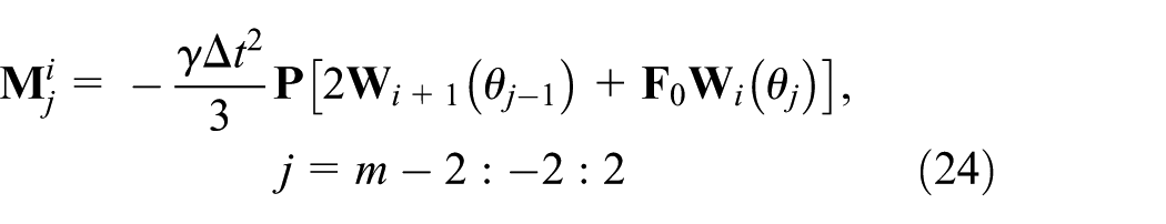
Making use of equation (13) in a similar procedure, the sub-matrices of the linear operator ${\mathbf{M}}_i$ of the corresponding $(m+n)$ -dimensional transition become

$${\mathbf{M}}_m^i=\mathbf{P}\{{\mathbf{F}}_0[\mathbf{I}+\frac{\mathrm{\Delta }t}{2}{\mathbf{B}}_i]-[\gamma \frac{3\mathrm{\Delta }{t}^2}{16}{\mathbf{F}}_0{\mathbf{W}}_i\left({\theta }_m\right)+\gamma \frac{9\mathrm{\Delta }{t}^2}{16}{\mathbf{W}}_{i+1}\left({\theta }_{m-1}\right)]\mathbf{D}\}$$

(28)

$${\mathbf{M}}_j^i=-\gamma \frac{9\mathrm{\Delta }{t}^2}{16}\mathbf{P}[{\mathbf{F}}_0{\mathbf{W}}_i\left({\theta }_j\right)+{\mathbf{W}}_{i+1}\left({\theta }_{j-1}\right)],j=m-1:-3:2$$

(29)

$${\mathbf{M}}_j^i=-\frac{3\gamma \mathrm{\Delta }{t}^2}{16}\mathbf{P}[3{\mathbf{F}}_0{\mathbf{W}}_i\left({\theta }_j\right)+2{\mathbf{W}}_{i+1}\left({\theta }_{j-1}\right)],j=m-2:-3:4$$

(30)

$${\mathbf{M}}_j^i=-\frac{3\gamma \mathrm{\Delta }{t}^2}{16}\mathbf{P}[2{\mathbf{F}}_0{\mathbf{W}}_i\left({\theta }_j\right)+3{\mathbf{W}}_{i+1}\left({\theta }_{j-1}\right)],j=m-3:-3:3$$

(31)

$${\mathbf{M}}_1^i=-\frac{3\gamma \mathrm{\Delta }{t}^2}{16}\mathbf{P}[3{\mathbf{F}}_0{\mathbf{W}}_i\left({\theta }_1\right)+{\mathbf{W}}_{i+1}\left({\theta }_0\right)]$$

(32)

$${\mathbf{M}}_0^i=-\frac{3\gamma \mathrm{\Delta }{t}^2}{16}\mathbf{P}{\mathbf{F}}_0{\mathbf{W}}_i\left({\theta }_0\right)$$

(33)

where

$$\mathbf{P}={[\mathbf{I}-\frac{\mathrm{\Delta }t}{2}{\mathbf{B}}_{i+1}+\gamma \frac{3\mathrm{\Delta }{t}^2}{16}{\mathbf{W}}_{i+1}\left({\theta }_m\right)\mathbf{D}]}^{-1}$$

(34)

Convergence of the methods

The error incurred on the application of the composite Simpson’s 1/3 rule is

$$E_{S1/3}\approx \frac{t_m-t_0}{180}{\left(\mathrm{\Delta }t\right)}^4\overline{f^{\left(\mathrm{iv}\right)}}$$

(35)

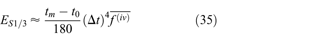
where $\overline{f^{\left(\mathrm{iv}\right)}}=\frac{1}{m}\sum _{j=0}^{m-1}{f}_{j+0.5}^{\left(\mathrm{iv}\right)}$ is the average value for the fourth-order derivative of $f(t)$ over the integration interval $[t_0,t_m]$ . Therefore, the error associated with the first-stage Simpson’s 1/3 rule is

$${\mathit{E}}_{S1/3}^{\left(1\right)}\left(t\right)\approx \frac{r}{180}{\left(\mathrm{\Delta }t\right)}^4\overline{\mathit{f}{}^{\left(\mathrm{iv}\right)}\left(t\right)}$$

(36)

where $\overline{\mathit{f}{}^{\left(\mathrm{iv}\right)}(t)}$ is the average temporal function for the fourth-order derivative of $\mathbf{W}(t,\theta )\mathbf{u}(t+\theta )$ with respect to $\theta$ over the integration interval $[-r,0]$ . Rather than equation (17), the exact solution becomes

$$\begin{array}{c}\multicolumn{1}{c}{\stackrel{·}{\mathbf{x}}\left(t\right)=\mathbf{Ax}\left(t\right)+\mathbf{B}\left(t\right)\mathbf{x}\left(t\right)}\\ \multicolumn{1}{c}{-\gamma \frac{r}{3m}\left[\begin{array}{c}\mathbf{W}(t,{\theta }_0)\mathbf{u}(t+{\theta }_0)+4\sum _{j=1:2:m-1}\mathbf{W}(t,{\theta }_j)\mathbf{u}(t+{\theta }_j)\hfill \\ \multicolumn{1}{c}{+2\sum _{j=2:2:m-2}\mathbf{W}(t,{\theta }_j)\mathbf{u}(t+{\theta }_j)+\mathbf{W}(t,{\theta }_m)\mathbf{u}(t+{\theta }_m)}\end{array}\right]}\\ \multicolumn{1}{c}{+{\mathit{E}}_{S1/3}^{\left(1\right)}\left(t\right)}\end{array}$$

(37)

On solving the first-order differential equation (37) and applying the second-stage NI, this error is propagated to

$${\mathit{E}}_{S1/3,i}^{\left(2\right)}=\underset{t_i}{\overset{t_{i+1}}{\int }}{e}^{\mathit{A}(t_{i+1}-s)}{\mathit{E}}_{S1/3}^{\left(1\right)}\left(s\right)\mathrm{d}s\approx \frac{\mathrm{\Delta }t}{2}({\mathbf{F}}_0{\mathit{E}}_{S1/3,i}^{\left(1\right)}+{\mathit{E}}_{S1/3,i+1}^{\left(1\right)})$$

Giving

$${\mathit{E}}_{S1/3,i}^{\left(2\right)}=\frac{r}{360}{\left(\mathrm{\Delta }t\right)}^5({\mathbf{F}}_0\overline{\mathit{f}{}^{\left(\mathrm{iv}\right)}\left(t_i\right)}+\overline{\mathit{f}{}^{\left(\mathrm{iv}\right)}\left(t_{i+1}\right)})=\mathcal{O}{\left(\mathrm{\Delta }t\right)}^5$$

The major error of the second-stage NI over the discrete interval $[t_i,t_{i+1}]$ is

$${\mathit{E}}_{\mathrm{TR},i}^{\left(2\right)}=\frac{{\left(\mathrm{\Delta }t\right)}^3}{12}[{\mathit{g}″}_{i+0.5}+\gamma \frac{r}{3m}{\mathit{h}″}_{i+0.5}]$$

where

$${\mathit{g}″}_{i+0.5}={\frac{d^2}{d{s}^2}\left[{\mathit{e}}^{\mathit{A}(t_{i+1}-s)}\mathbf{B}\left(s\right)\mathbf{x}\left(s\right)\right])}_{s=t_{i+0.5}}$$

and

$${\mathit{h}″}_{i+0.5}=\frac{d^2}{d{s}^2}\{{e^{\mathit{A}(t_{i+1}-s)}\left[\begin{array}{c}\mathbf{W}(s,{\theta }_0)\mathbf{u}(s+{\theta }_0)+4\sum _{j=1:2:m-1}\mathbf{W}(s,{\theta }_j)\mathbf{u}(s+{\theta }_j)\hfill \\ \multicolumn{1}{c}{+2\sum _{j=2:2:m-2}\mathbf{W}(s,{\theta }_j)\mathbf{u}(s+{\theta }_j)+\mathbf{W}(s,{\theta }_m)\mathbf{u}(s+{\theta }_m)}\end{array}\right]\})}_{s=t_{i+0.5}}$$

The local discretization error of the method becomes

$${\mathit{E}}_i={\mathit{E}}_{S1/3,i}^{\left(2\right)}+{\mathit{E}}_{\mathrm{TR},i}^{\left(2\right)}=\frac{{\left(\mathrm{\Delta }t\right)}^3}{12}[{\mathit{g}″}_{i+0.5}+\gamma \frac{\mathrm{\Delta }t}{3}{\mathit{h}″}_{i+0.5}+\frac{r}{30}{\left(\mathrm{\Delta }t\right)}^2({\mathbf{F}}_0\overline{\mathit{f}{}^{\left(\mathrm{iv}\right)}\left(t_i\right)}+\overline{\mathit{f}{}^{\left(\mathrm{iv}\right)}\left(t_{i+1}\right)})]$$

(38)

If the trapezoidal rule was used to handle the distributed delay rather than Simpson’s rule, the propagated error becomes

$${\mathit{E}}_i=\frac{{\left(\mathrm{\Delta }t\right)}^3}{12}[{\mathit{g}″}_{i+0.5}+\gamma \frac{\mathrm{\Delta }t}{2}{\mathit{h}″}_{i+0.5}+\frac{r}{2}({\mathbf{F}}_0\overline{\mathit{f}″\left(t_i\right)}+\overline{\mathit{f}″\left(t_{i+1}\right)})]$$

(39)

where, in this case

$${\mathit{h}″}_{i+0.5}=\frac{d^2}{d{s}^2}\{{e^{\mathit{A}(t_{i+1}-s)}\left[\begin{array}{c}\mathbf{W}(s,{\theta }_0)\mathbf{u}(s+{\theta }_0)\hfill \\ \multicolumn{1}{c}{+2\sum _{j=1}^{m-1}\mathbf{W}(s,{\theta }_j)\mathbf{u}(s+{\theta }_j)+\mathbf{W}(s,{\theta }_m)\mathbf{u}(s+{\theta }_m)}\end{array}\right]\})}_{s=t_{i+0.5}}$$

The local discretization error is, therefore, proportional to the cubic power of the discretization step $\mathrm{\Delta }t$ in both the cases, that is, ${\mathit{E}}_i=\mathcal{O}(\mathrm{\Delta }t{)}^3$ . By comparing equations (38) and (39), we can see that the weight of $(\mathrm{\Delta }t{)}^3$ is smaller when Simpson’s rule is used to handle the distributed delay rather than the trapezoidal rule. Thus, the proposed methods are expected to be only slightly more accurate and convergent than the pioneering two-stage NI method, which was proposed and proved in Ozoegwu ¹⁴ to be of the same level of accuracy as the well-accepted first-order semi-discretization method. ¹² Since the exact analytical forms of h and f are not known, numerical simulation will be needed to gauge the extent of the expected rise in accuracy with higher order first-stage NI rules against the backdrop of the Runge phenomenon. It must be noted that the sparseness of the monodromy matrix does not change with higher order first-stage NI rules, thus rise in computational time is not expected but a slight rise in computational time is expected since the diversity of the first row of sub-matrices rises with higher order first-stage NI rules. From application point of view, it can be concluded that it may not be necessary to increase the first-stage NI rule beyond the first order since according to theoretical error analysis that will result in minor improvement in accuracy.

Numerical investigation

The properties of the computer used for numerical calculations are as follows: processor, Intel(R) Core(TM) i7-5500U CPU at 2.4 GHz; installed memory, 8GB; and system type, 64-bit Operating System, x64-based processor.

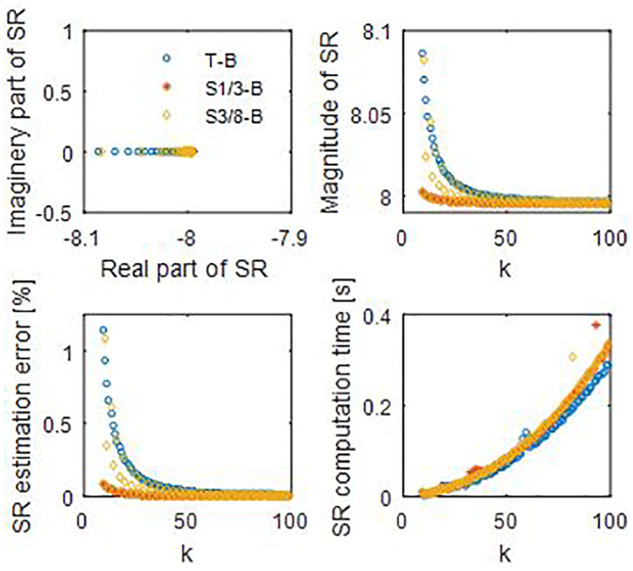
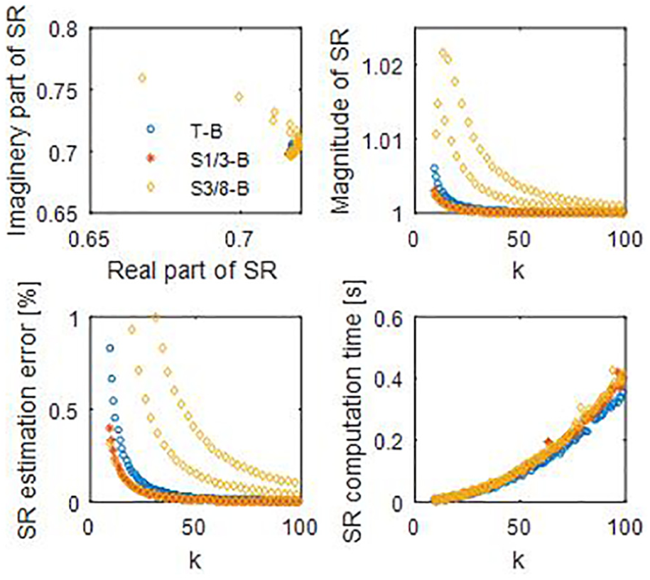
The DIDE in equation (15) with $\mathrm{w}(\theta )=-(\pi /2)\sin (\pi \theta )$ is used for numerical investigation. The numerical rate of convergence and computational time plots are given in Figures 1–3. In each of the figures, the subplots (2, 2, 1), (2, 2, 2), and (2, 2, 3) are the various numerical rate of convergence plots. In the subplot (2, 2, 1) of Figure 1, the convergence of the spectral radius (SR) on the Argand plane as k changes from 9 to 99 is plotted. A very convergent method will have an SR which tends to remain at a spot as k varies. The meaning is that in Figure 1, which is plotted at the unstable point $\delta /{\pi }^2=5$ and $\gamma /{\pi }^2=-50$ , the proposed Simpson’s 1/3-based (S1/3-B) two-stage NI method is the most convergent. The subplot (2, 2, 2) shows the asymptotic convergence plot of the SR magnitude which is seen to re-echo the result of subplot (2, 2, 1) where S1/3-B method is the most convergent. This subplot also clearly shows that the parameter point is unstable being that the asymptotic value has a magnitude greater than unity. The subplot (2, 2, 3) shows the plot of percentage error of SR magnitude relative to a reference (very accurate) SR magnitude computed at k = 240. This subplot is seen to re-echo the result of subplot (2, 2, 1) where S1/3-B method is the most convergent. For example, when k = 15, the percentage error of the pioneering trapezoidal-based (T-B), S1/3-B, and the proposed Simpson’s 3/8-based (S3/8-B) methods are, respectively, 0.43%, 0.04%, and 0.35%. Also, when k = 30, the percentage error of the T-B, S1/3-B, and S3/8-B methods are, respectively, 0.12%, 0.01%, and 0.11%. This confirms that the S1/3-B method is very convergent. The subplot (2, 2, 4) shows the trend of SR computational time as k changes from 9 to 99. The fact that the S1/3-B method is the most convergent is further emphasized with plots at the parameter coordinates [ $\delta /{\pi }^2$  = 20, $\gamma /{\pi }^2$  = 12.5] and [ $\delta /{\pi }^2$  = 13, $\gamma /{\pi }^2$  = 5] shown, respectively, in Figures 2 and 3. The fact that the proposed S1/3-B method is more convergent than the T-B method agrees with the result of error analysis in the preceding section. It is noteworthy from subplot (2, 2, 2) of each of the figures that the parameter points are both stable being that the asymptotic value has a magnitude not greater than unity (the former being stable only in Lyapunov’s sense). But the fact that S1/3-B is numerically more accurate than S3/8-B means that the first-stage NI rule should not go beyond the second order. The subplot (2, 2, 4) of each of Figures 1–3 confirm that expectation from error analysis that higher order first-stage NI rules will cause negligible rise in computational time.

Figure 1.

Subplots of the numerical rate of convergence at the unstable point $\delta /{\pi }^2$  = 5 and $\gamma /{\pi }^2$  = –50. The legend in subplot (2, 2, 1) applies to the other subplots.

Figure 2.

Subplots of the numerical rate of convergence at the critically stable point $\delta /{\pi }^2$  = 20 and $\gamma /{\pi }^2$  = 12.5. The legend in subplot (2, 2, 1) applies to the other subplots.

Figure 3.

Subplots of the numerical rate of convergence at the stable point $\delta /{\pi }^2$  = 13 and $\gamma /{\pi }^2$  = 5. The legend in subplot (2, 2, 1) applies to the other subplots.

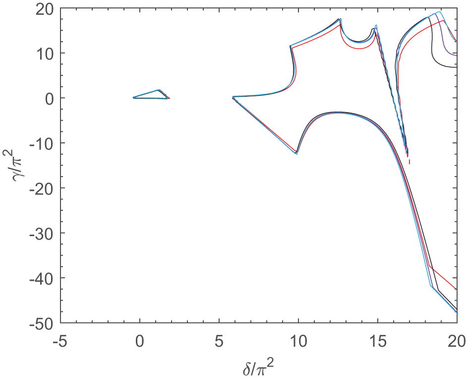
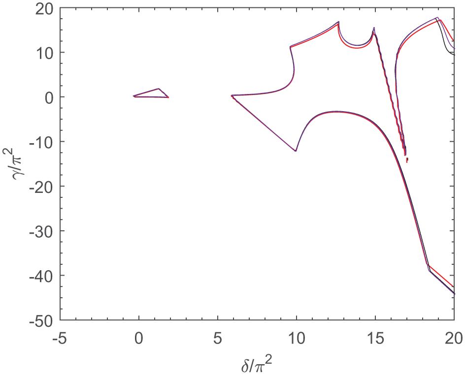
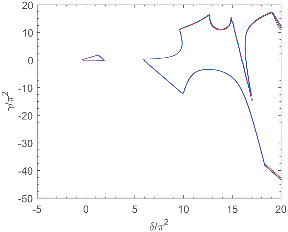
By making use of approximation parameter $k=60$ on a $200\times 300$ gridded plane of $\delta /{\pi }^2$ and $\gamma /{\pi }^2$ , a reference stability diagram is identified using the T-B two-stage NI method of the work. ¹⁴ The reference stability diagram is the red curve in Figures 4–6. It is important to note that the domain enclosed within the red curve is stable, while that external to the curve is unstable. This is collaborated by the simulations in Figures 1–3, that is, the classification of the parameter points as unstable, critically stable, and stable is seen to agree with the stability curve. In Figure 4, the pioneering T-B, the proposed S1/3-B, and the proposed S3/8-B two-stage NI methods are used to compute the stability curves at $k=6$ on the same axes as the reference stability curve. With the exception of Figure 4, which tended to be inconclusive, the proposed methods only slightly improved computational accuracy. These results agree with the theoretical error analysis that from application point of view, it is not necessary to increase the first-stage NI rule beyond the first order (trapezoidal rule) though the best results are expected at second order (Simpson’s 1/3 rule).

Figure 4.

Reference stability boundary (red curve) at $k=60$ for equation (15) with $\mathrm{w}(t,\theta )=-(\pi /2)\sin (\pi \theta )$ , $\kappa =0.1$ , $T=0.5$ , and $ϵ=40$ identified after 12,134 s CT using the trapezoidal-based two-stage NI method. The black, purple, and blue stability boundaries are, respectively, identified at $k=6$ using the trapezoidal-based, Simpson’s 1/3-based and Simpson’s 3/8-based two-stage NI methods after the respective CT of 289.3496, 346.3947, and 365.0041 s.

Figure 5.

The black and purple stability boundaries are, respectively, identified at $k=10$ using the trapezoidal-based and Simpson’s 1/3-based two-stage NI methods after the respective CT of 767.7280 and 840.0205 s. Simpson’s 3/8-based two-stage NI methods cannot be used because $k=10$ is not a multiple of 3.

Figure 6.

The black, purple, and blue stability boundaries are, respectively, identified at $k=15$ using the trapezoidal-based, Simpson’s 1/3-based, and Simpson’s 3/8-based two-stage NI methods after the respective CT of 856.6793, 972.2129, and 1102.4 s.

Conclusion

Alternative methods of the two-stage NI approach, introduced in Ozoegwu ¹⁴ for stability identification of distributed-delay oscillators, were compared theoretically and numerically for accuracy and computational time. This was done using tensor-based higher order NI rules to handle the distributed delay. As in the pioneering two-stage NI approach, the additional methods formulated here used the trapezoidal rule for the second-stage NI. The second-stage NI is needed for creating discrete transition and constructing the monodromy matrices of the approach. It was found that the propagated local discretization error is of order $\mathcal{O}(\mathrm{\Delta }t{)}^3$ irrespective of whether the distributed delay was handled with the trapezoidal rule or higher order NI rules, but $(\mathrm{\Delta }t{)}^3$ is less weighted when higher order NI rules are used, meaning that a slightly higher accuracy results from using higher order first-stage NI rules. The higher accuracy was verified using the following numerical convergence techniques: Argand plane convergence rate, asymptotic convergence rate, percentage error convergence rate, and comparative stability computation. Combining both theoretical and numerical results led to the conclusion that from application point of view, it is not necessary to increase the first-stage NI rule beyond the first order (trapezoidal rule) though the best results are expected at second order (Simpson’s 1/3 rule).