
Abstract
This paper describes the kinematics and dynamics modelling of a mechanical system consisting of a spherical inverted pendulum whose base is mounted on a parallel planar mechanism, better known as a five-bar mechanism. The whole mechanism has four degrees of freedom, but it has only two actuators and so it is an under-actuated system. The nonlinear dynamics model of the complete system is first obtained using a non-minimal set of generalized coordinates, and then a reduced equivalent model is computed. To validate this approach, the reduced model is linearized and simulations are carried out, showing the stabilization of the system with a simple LQR controller. Experimental results on an academic prototype are also presented.
Introduction
The problem of balancing an inverted pendulum has attracted the attention of control researchers in recent decades [1]. There exist a wide variety of inverted-pendulum-type systems, such as the pendubot, the acrobot, the pendulum on a cart, the inertial wheel pendulum and the Furuta pendulum (see, e.g., [2–5]). All these systems are under-actuated [6], that is, they are systems with fewer actuators than degrees of freedom (dof). The degree of under-actuation is indeed the difference between the number of dof and the number of actuators. All the examples of inverted pendulums mentioned above have a degree of under-actuation of one.
This paper deals with the modelling and control of a spherical inverted pendulum (SIP), which is another member of the family of inverted pendulum systems with degree of under-actuation of two.
The system consists of a rigid rod coupled in its base to an under-actuated universal joint in such a way that the extreme of the rod moves over a spherical surface with its centre at the base of the rod (see Figure 1). As such, through the motion of the base of the pendulum on the horizontal plane it is possible to balance the extreme of the rod in its upright position.

Spherical inverted-pendulum on a five-bar mechanism
The SIP has been studied by numerous researchers (see [7 – 11]). The interest in studying the SIP is due to its mathematical model, which is considered as a simplified model of a rocket-propelled body or a building, such that it can be used for the control of the position of a rocket, for the control of the oscillations of buildings, or simply for the study of new control techniques.
According to [12], there exists a classification of SIP-type systems, depending on the mechanism used to stabilize the SIP, which can be:
In this document, it is considered that the motion of the base of the SIP is controlled by means of a five-bar mechanism (FBM), which is a well-known closed-chain mechanism. Such a system has become common, due to the existence of a commercial prototype for academic and research purposes (see [15]). The complexity of the mathematical model and control of this system (SIP+FBM) is due in great measure to the kinematic constraints imposed by the closed-loop of the FBM.
To the best of the authors' knowledge, the only work dealing with the modelling and control of a similar SIP+FBM mechanism is [12]. In that work, the authors consider the system as a linear parameter variable (LPV) system with structured additive perturbation. This paper uses a different approach to obtain the complete non-reduced dynamics model of the same system.
The equations that govern the motion of any mechanical system must take into account the kinematic constraints among all the elements of the system. For open-chain mechanisms (OCMs), this is a direct task and there are several methods to do it, producing a set of ordinary differential equations (ODEs). Qn the other hand, for a closed-chain mechanism (CCM) the existence of loops originates simultaneous algebraic constraint equations which cannot be solved explicitly. Therefore, the equations of motion for a CCM are a set of differential-algebraic equations (DAEs) [16].
We should mention that in our laboratory there exists a prototype of a SIP+FBM with some parts of the commercial system [15]. The motor drives that we use to control the system allow us to work in current (torque) mode [17].
The purpose of this paper is threefold. First, we recall the theory concerning the modelling of mechanisms with constraints, and specifically the projection methods for simplifying the resulting equations. Secondly, we apply such methods for obtaining the kinematics and dynamics model of the SIP+FBM system. At the end, we show the validity of such a model by implementing an LQR controller in both simulations and experiments in our prototype.
The remainder of this paper is organized as follows. Section 2 is devoted to the modelling of constrained systems in general. The kinematics and dynamics models of the system under study are obtained in Section 3. The validation of the models via simulations/experiments with an LQR controller is shown in Section 4, while final conclusions are given in Section 5.
It is worth mentioning that most of the theory presented in this section is not novel, and can be found, for example, in [18] and [16].
Kinematics model
Consider a CCM with m joints but with only n(n<m) dof; then, there should exist p=m−n holonomic constraints which allow the reduction of the order of the system from m to n; in others words, if we choose n independent joint variables there must exist p dependent joint variables.
Let
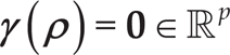
so that, as a result, it should be possible to express β as a function of q, i.e.,

The direct kinematics problem consists in finding expressions for the pose (i.e., position and orientation) variables of an element of interest of the CCM, described by the vector x in terms of the actuated joint variables; this can be expressed as

In addition, by taking the time derivative of the previous equation we get the so-called differential kinematics equation

where
On the other hand, the inverse kinematics problem consists in establishing the value of the actuated joint coordinates that correspond to a given pose of the element of interest, and can be expressed as
The inverse kinematics problem can be solved in general form by geometric or analytic approaches, such as those mentioned in [19].
As mentioned in [20], the dynamics model of CCMs using either the Newton-Euler or the Euler-Lagrange methodology is traditionally obtained by cutting the closed loops to obtain systems with open chains and/or tree-type structures, so that it is possible to write a set of ODE s for such chains in their corresponding generalized coordinates. The solution to these equations requires satisfying additional algebraic equations guaranteeing the closure of the cut-open loops. To this end, some Lagrange multipliers (which physically represent the forces due to the constraints) are employed. The resulting formulation, often referred to as a descriptor form, yields a system of DAEs which, in general, cannot be solved employing conventional ODE techniques.
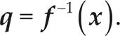
The most general form of a differential-algebraic system of n equations is that of an implicit differential equation [21]
where u ∊ ℝn is the vector of generalized coordinates, t is the time variable, and
System (2) has a differential index μ if μ is the minimal number of analytical differentiations

such that the system of equations (3) allows us to extract, by algebraic manipulations, an explicit ordinary differential system u = ϕ(u) (which is called the 'underlying' ODE)
According to [16], if the differential index is 1 or 2, it is usually possible to differentiate the constraint equation with respect to time once (index 1) or twice (index 2) to produce an equivalent ODE (a process sometimes called index reduction) and to achieve satisfactory results using standard numerical methods for ODEs. If the differential index is greater than 2, standard numerical methods frequently fail to converge, and sometimes converge to incorrect solutions.
These DAEs resulting from the dynamical analysis of CCMs have a differential index of 3. Several methods have been proposed in the literature in order to transform them into a set of ODEs with fewer generalized coordinates so that they can be solved analytically or numerically.
The most important of such methods are [20]:
Direct elimination, where the surplus variables are eliminated directly, using the algebraic constraints given by the kinematics, to explicitly reduce index-3 DAEs to ODEs in a minimal set of generalized coordinates (see [22]). Explicit Lagrange-multiplier computation, using the unknown accelerations computed from the index-1 DAEs formed by appending the acceleration constraints (computed by differentiating the original constraint) to the system equations (see [23] and [24]). Projection of the dynamics onto the tangent space of the constraint manifold, where the constraint-reaction dynamics equations are taken into the orthogonal and tangent sub spaces of the vector space of the system generalized velocities. A family of choices exist for the projection, as surveyed by [25] and [26].
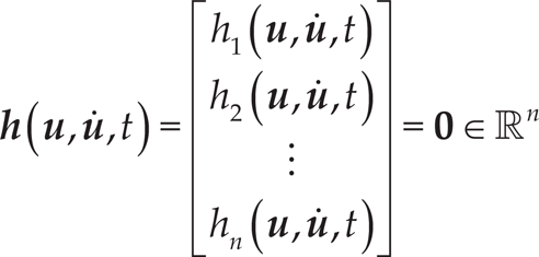
The dynamics model of a mechanism of n dof, with m generalized variables (m>n), and subject to p=m−n holonomic constraints, can be represented by means of the following index-3 DAEs


where the Lagrangian

being

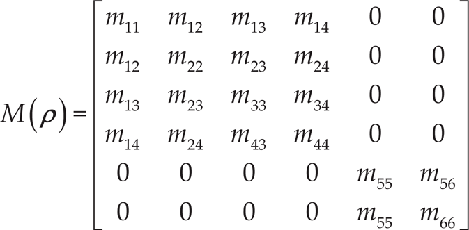
where M(ρ)∊ℝm×m is the inertia matrix,
Moreover, as explained in [27], the following properties are satisfied for M(q) and g(q)


With the matrix M(ρ), it is possible to compute the matrix

where Mij(ρ) denotes the ij th element of the inertia matrix M(ρ). Indeed, the kj th element

The projection of dynamics (7) onto the tangent space of the constraint manifold (5) consists on finding a matrix R(ρ)∊ℝm×m whose column space belongs to the null space of D(ρ), i.e., D(ρ)R(ρ) = 0. All feasible dependent velocities

The matrix R(ρ) for a particular system depends on the selection of the generalized coordinates ρ, the independent variables ρ (which can be extracted from ρ through a function α such that ρ = α(ρ)), and the constraints γ(ρ). Appendix A describes a procedure to obtain R(ρ) starting from these relations.
Using such a matrix R(ρ), it is possible to reduce the system (7) to a new index-1 DAE system
where
In this section, the kinematics and dynamics models of a SIP+FBM system, as the one shown in Figure 2, are obtained. This figure also shows the frames attached to each extreme of the FBM (Σ0 and Σ0), as well as those of the base (Σb) and the extreme (Σp) of the pendulum. In general, Σi is considered to be formed by the axes xi,yi, zi.

Schematic diagram of the SIP+FBM
The angles θ and φ indicate the orientation of the extreme of the pendulum with respect to the frame Σb;θ is the angle that rotates with respect to the axis yb and φ is the angle that rotates with respect to the axis xb.
The angles q1 and q2 of the active joints of the FBM determine its configuration. The angles β1 and β2 of the passive joints depend upon q1 and q2. For the purposes of analysis, in this paper the vector of independent joint variables is defined as
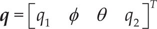
and the vector of pose variables of the pendulum as

The lengths of the four mobile links are considered equal to L, and the length of the pendulum is Lp.
Direct kinematics model
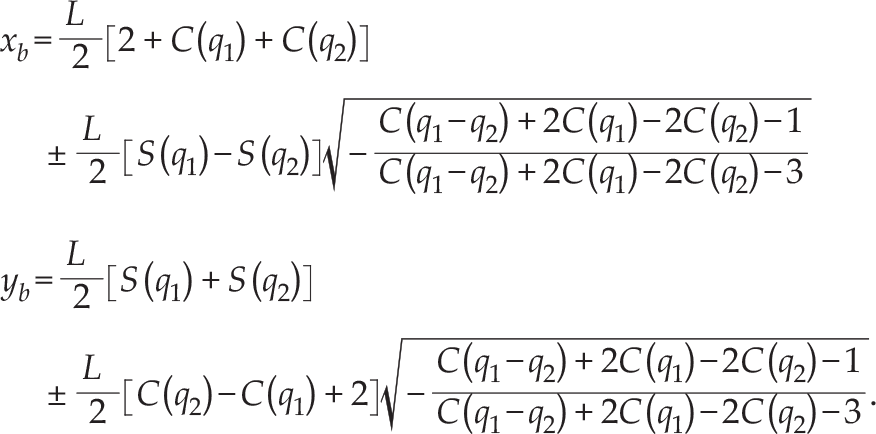
The problem of direct kinematics is reduced to find the coordinates of the intersection points of a circle of radius L with C1 and C2 as centres, as shown in Figure 3(a), the equations of which are

where the notations S(·) and C(·) are used for sin(·) y cos(·), respectively. Using a software tool such as MATLAB, it is possible to find the following two solutions for xb and yb

Geometric relations of the FBM
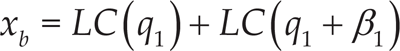
Furthermore, from Figure 3 (b) it is possible to obtain the following relations

From Figure 3 (a), the following expressions can be defined


and on the other hand, from Figure 3 (b) it is observed that

where

and also

As such, making some algebraic operations with equations (16), (17) and (20)–(22), it yields

Following a similar procedure, but starting from equations (18) and (19), we get

Taking the time derivative of (16)–(19) for i = 1,2, we obtain


As such, multiplying the equations (23) and (24) by cos(qi + βi) and sin(qi + βi), respectively, and adding the results, we further obtain

and by taking i = 1,2 in (25), we find the matrix equation that relates the operational velocities

Now, from the differential kinematics equation (1), considering (14) and (15), we can show that

Moreover, from (23) and (24), we get

which leads to
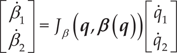
where
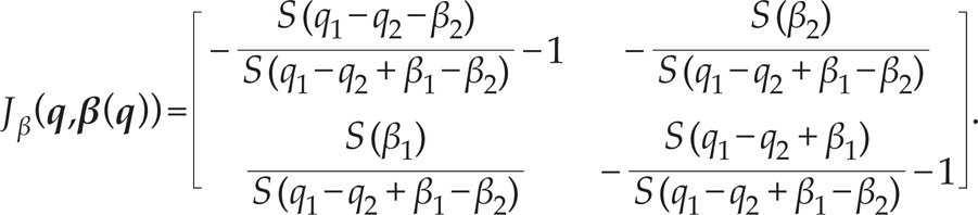
Equation (26) establishes the relation between the actuated and passive joint velocities of the FBM.
Following the approach proposed in [18], let us consider that the system in Figure 2 is cut out at point C, producing two separated OCMs: one with four dof formed by the left leg of the FBM and the SIP, and one with two dof formed by the right leg. Now, it is possible to use as a vector of generalized variables
In the following, we show how to obtain each of the elements of equation (7) and then how to get the reduced system (13).
The total kinetic energy of the system can be divided in:
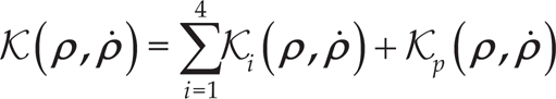
where Ki is the kinetic energy associated with the link i of the FBM and Kp is the kinetic energy associated with the pendulum; Ki and Kp can be obtained by [27]
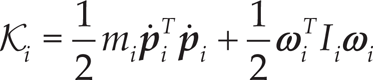

where
The position vectors of the centres of mass of each link for the FBM are

where lci is the distance from a joint to the centre of mass of link ii as shown in Figure 2. The position vector of the centre of mass of the pendulum is described by the equation

where

As the FBM is located in the XY plane, the angular velocities for each link can be defined as

while the angular velocity of the pendulum with respect to frame Σ0 is given by [28]
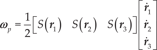
where S (·) is a skew-symmetric matrix such that, for a vector

and the vectors r1,r2 and r3 are the columns of the rotation matrix from frame Σp with respect to frame Σ0, the elements of which are
Therefore, using (30), we get

Moreover, in equation (28) we require the mass of each link of the FBM as well as the matrix of inertia moments with respect to a coordinate frame that passes through the centre of mass. Again, taking into consideration that the FBM moves in the horizontal plane, only the inertia moments along the z0 axis are of interest for the links, namely I1I2,I3 and I4. For the SIP, the matrix of the inertia moments is given by

It is possible to use software for symbolic computing to obtain the matrices of the dynamics model (7). In order to obtain the matrix M(ρ), the total kinetic energy
where
Using expressions (10) and (11), we can compute

where each element of the matrix is given by
with
Finally, for the vector of gravitational forces, the total potential energy (which only depends of the potential energy of the SIP) is obtained using
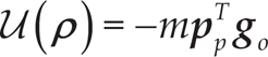
where g0 is a vector that indicates the gravitational acceleration with respect to Σ0. Then, by applying (9) we get

hence

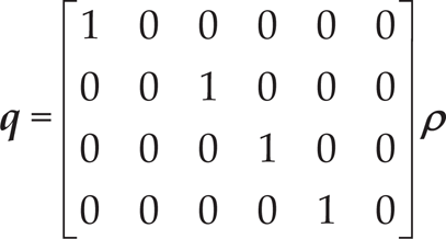
The constraints of the system are given by

and the relation q = α(ρ) is simply defined by
Thus, matrix R(ρ), which satisfies (12), is defined as
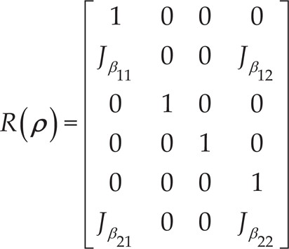
where
The matrices of the reduced model of the system (7) are defined as

where the components of each one are given by
and the vector of gravitational forces is defined as

Description of the prototype
The prototype in our laboratory was integrated from different commercial components. Instead of acquiring the whole Quanser system in [15], we only purchased the FBM and the SIP as individual parts. An aluminium base for the mechanism was made, and two motors with encoders (model 2224U006 from Faulhaber) were coupled to it as the actuators for the FBM. Some servo amplifiers (model BE15A8 from Advanced Motion Control (AMC)) were employed to operate the motors in current (torque) mode. A power module (model PS2X3W24, also from AMC) was used to supply the required power.
The dynamical parameters for the FBM and the SIP were estimated from the CAD model of these elements using SolidWorks and considering the actual masses of each of their component parts.
To control the mechanical system, we employ MATLAB/Simulink and a Sensoray 626 data acquisition board as an interface for sending the control signals to the motor drives and receiving the encoder measurements.
Figure 4 shows a schematic diagram of the whole system and Figure 5 shows a photograph.
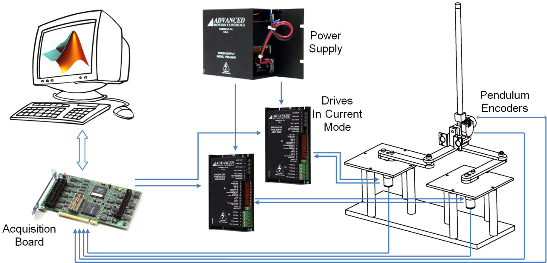
Schematic diagram of the SIP+FBM system

Photograph of the experimental prototype
Most of the references that treat with spherical pendulums (e.g., [8, 14, 7]), and including the manufacturer of the commercial version of this mechanism [15], assume that the angles φ and θ of the pendulum are almost zero. Therefore, the system can be decoupled in two systems, and a linearized dynamics model is obtained for each system in order to apply a linear controller.
We now present the linear model of the complete system (13) in order to apply an LQR controller.
Model linearization
Considering

where the kinematic relations in Section 3.1 can be used to compute
Considering

where the constant matrices A and B are defined as

with
It is well–known in literature that system (32) can be stabilized using a linear state–feedback control law given by

And if K is chosen such that

where P is found by solving the algebraic Riccati equation

using some positive definite matrices of proper dimensions Q and P, then we ensure that the cost function

is minimized. Such is known as an LQR controller.
In this section, we show the evaluation of the SIP+FBM system in a closed loop with an LQR controller. Both simulations and experiments are tested.
Simulations
In order to apply the LQR controller to the system (13), we consider for the parameters of the system the values that are shown in Table 1. These parameters were estimated using conventional identification procedures for our academic prototype.
Considering that the matrices Q and G of (34) are defined by

the K matrix is given by

Parameters of the SIP+FBM mechanism

Parameters of the SIP+FBM mechanism
with gains k11 = −0.6236, k13 = −4.9548, k15 = −0.2669, k17 = −0.6912, k22 = 4.7337, k24 = −0.6236, k26 = 0.6591, k28 = −0.2618.
The position errors of the independent variables are given by
The initial conditions were considered as

Position error of q1 and q2 (simulation)

Position error of φ and θ (simulation)
We also carried out some experiments in our prototype. We considered using the same control gains as in the simulation. A sampling period of 1ms was employed. Initial conditions for the experiments were assumed to be as close as possible to the equilibrium point. Figure 6 shows the time evolution of
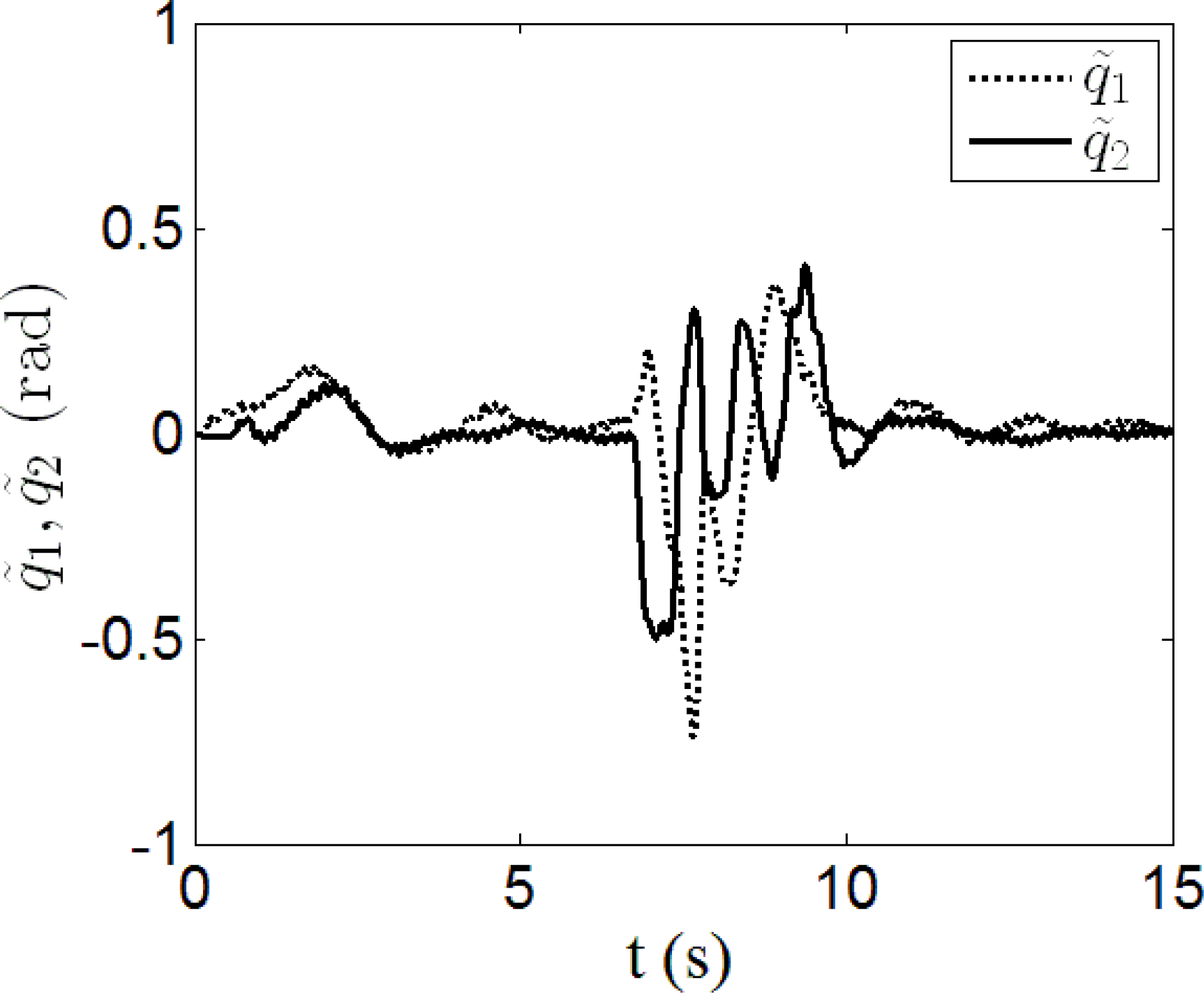
Position error of q1 and q2 (experiment)
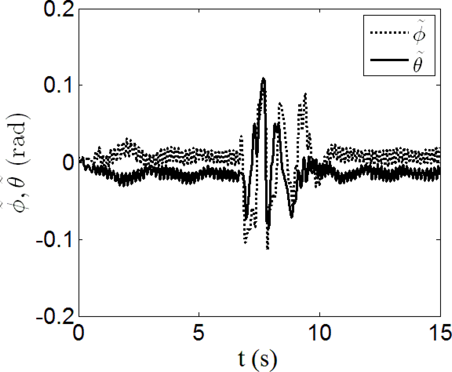
Position error of φ and θ (experiment)

Applied torque for the joint of q1

Applied torque for the joint of q2
This document presented a way of obtaining the kinematics and dynamics model of a system consisting of an inverted pendulum mounted on a FBM. The dynamics model is obtained in terms of a non-minimal set of generalized coordinates and then it is reduced using an approach proposed in the literature. In order to validate this resulting model, we carried out some simulations and experiments on a didactic prototype we have in our laboratory. The resulting model is novel, however, since it uses no simplifications as in [12].
Footnotes
6.
This work was partially supported by PROMEP, DGEST and CONACYT (grant 60230). The authors would also like to thank Jaqueline Bernal for her support in acquiring a better understanding of DAEs.
Appendix
Computation of matrix R(ρ)
Consider a closed-chain mechanism which is described by means of the vector ρ∊ℝm of generalized coordinates, from which we can extract the vector ρ∊ℝn of independent coordinates using the function
and let
be the vector of holonomic constraints of the system.
The matrix R(ρ)∊ℝm×n, which allows the transformation of the system dynamics from an index-3 DAE to an index-1 DAE, as described in Section 2, can be computed using the following expression
where
Given (35), it can be proved that
Now, it is worth noticing that we can write
where
and as Ψ(ρ) is full-rank, then it is possible to also write
which agrees with the definition R(ρ) found in [18].