Obstacle Avoidance Path Planning of Planar Redundant Manipulators Using Workspace Density

Abstract

This paper presents a new approach to generate the workspace of planar redundant manipulators based on the workspace density of a single link. The workspace density of planar serial redundant manipulators can be computed efficiently by using the concept of the Fourier transform for the group of rigid-body motions of the plane and the convolution theorem. For manipulators using discrete actuation, it is important to study not only the shape of the workspace, but also the density of reachable poses in the workspace. In this paper, we focus on using the workspace density to calculate collision-free paths in complex environments with multiple obstacles in the workspace of the manipulator. This paper presents the algorithm and demonstrates it effectiveness using simulation results.

1. Introduction

Because of the advantages of redundant manipulators, such as dexterity and the ability to avoid obstacles, they are widely used in industry and the medical robotics field. In the research field of redundant manipulators, methods to generate the workspace have been studied extensively. The manipulator workspace is defined as the space of points reachable by the end-effector. Many researchers have been focused on different approaches to generate the shapes and boundaries of workspace. Traditionally, three methods have been used to generate the workspace of manipulators: (1) geometric methods which are only applicable to simple manipulator structures, and not for general structures; (2) numerical sampling methods which are simple algorithms. Due to the main disadvantage of this algorithm, low efficiency, it is mostly used for qualitative analysis and geometric validation; (3) analytic methods in which closed-form functions are used to describe the workspace.

The topic of computing the workspace of manipulators has drawn a lot of attention by researchers since the last half century. Many efficient approaches have been developed for various types of robotic manipulators. The authors of [1] presented the efficient geometric algorithms to simulate the workspace of redundant manipulators. A classification based on the workspace topology defined by cusps and nodes that appear on singular curves was used by [2].

The authors of [3] proposed a numerical algorithms to map the boundaries of workspace. An initial point on the boundary was found by a numerical method in that paper. The Monte Carlo method was used by [4] to generate the workspace of robotic manipulators. Two numerical formulations were compared in [5]. One numerical formulation was based on continuation methods to map the boundary of manipulator workspaces. The other one was based on a similar rank-deficiency criteria to yield the boundary of workspace. The authors of [6] presented a partition scheme to obtain the orientation workspace of a 3-degrees of freedom (DOF) spherical parallel manipulator. The authors of [7] proposed a method to determine the boundary for general manipulator workspaces.

An analytic method was proposed by [8] and [9] which described the boundary of open-chain-manipulator workspace. The algebraic formulation was a function of the dimensional parameters of the manipulator and the revolute joint angle of the end-effector.

The authors of [10] proposed the concept of a convolution product of real-valued functions on the Special Euclidean group which was applied to generate the workspace of discretely actuated manipulators. Then the authors developed a diffusion method to generate the workspace of hyper-redundant manipulators in [11] and [12]. This algorithm generated the workspace by solving the diffusion equation which based on the length and kinematic properties of manipulators. The authors of [13] presented a mathematical model to generate the workspace density based on the properties of the Fourier transform and the inverse Fourier transform.

Many investigations have focused on obstacle avoidance of redundant manipulators which have many different paths to achieve desired tasks in their workspace. The authors of [14] proposed a novel continuous genetic algorithm along with the distance algorithm for solving collisions-free path planning problem for robot manipulators. In [15], the path planning function was considered as a sequence of a nonlinear programming problem which minimized the distance between the current location of the end-effector and a desired location. The authors added two penalties to the path planning function to ensure that the manipulator did not collide with or cross over any obstacle. The trajectory planning of redundant manipulators which achieved tasks within the enclosed workspace was studied in [16]. The authors of [17] presented the obstacle avoidance problem of spatial hyper-redundant manipulators in known environments. They employed harmonic potential functions to achieve obstacle avoidance and generated the potential of any arbitrary shaped obstacle in three-dimensional space with a modified method. The authors of [18], required manipulators to remain approximately tangent to the curves which were given by B-spline curves based on an approximated path. The basic idea of [19] used harmonic potential fields to find a smooth path which consisted of points close enough to each other. Then manipulators reached the goal by keeping the tip of each link on these path points. In [20], the authors studied the complexity of fractional dynamics of the chaotic response based on Fourier transform and wavelet analysis. Their perspective of the chaotic phenomena permitted the development of superior trajectory control algorithms.

With the development of intelligent control, novel approaches such as neural network and genetic algorithms were used to solve the path planning of manipulators. [21] proposed a neural network adaptive controller to obtain the path planning of redundant robot manipulators. The parameter adaptation algorithm was based on the stability study of the closed loop system which used Lyapunov approach with configuration parameter of manipulators. The authors of [22] presented a adaptive neural controller constructed in task space based on an optimization strategy using joint displacement energy and internal penalty functions that consider the positions of the obstacle. The closed-loop pseudo-inverse method and genetic algorithms were combined in [23].

Each methodology contains certain advantages and disadvantages in the workspace generation and the path planning of robot manipulators. In this paper, the workspace density of planar serial revolute manipulators can be efficiently computed. We solve the path planning problem for planar serial revolute robot arms based on the “closed-form” workspace density. This approach selects a solution from a very large discrete set using workspace density as an evaluation. The planar serial revolute manipulators have optimal flexibility in the area of maximal values of workspace density function.

2. Workspace density

Our paper uses a similar approach to generate workspace as [24]. They employed closed-form convolution of real-valued functions on the Special Euclidean Group for generating workspaces. A method based on the Fourier transform of the discrete-motion group for computing the configuration and workspaces of robot manipulators was proposed in [13],[25],[26].

2.1 Definition of workspace density

Generally speaking, the definition of a manipulator workspace is the space of rigid-body motions where the end-effector of robot manipulator can reach. Assume that a robot manipulator has N links and each joint has M states. Then the number of the states that the end-effector can reach is K = M^N.

The workspace W of a planar robot manipulator is divided into small boxes (voxels) of equal size Δx, Δy, Δθ. The workspace density ρ assigns the number of points within each box of the workspace W that are reachable, normalized so as to be a probability density.

$\rho \text{(box)}=\frac{\#\text{of reachable points in box}}{\text{(total \# of points)}\cdot \text{(volume of the box)}}$

(1)

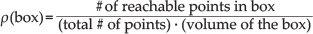
This density is a probabilistic measure of the positional and orientational (pose) which describes accuracy of the end-effector in a considered area of the workspace. The higher the density of a point in the box, the more likely we expect the manipulator to be able to reach a pose.

As established in [27], when a robotic manipulator is separated into the lower and the upper segment, convolving the densities of each segment will result in the density of the whole manipulator. Generally speaking, if f₁(g) is the density of the lower segment and f₂(g) is the density of the upper one, then the density of the whole manipulator will be

$(f_1*f_2)\left(g\right)={\displaystyle {\int }_G}{f}_1\left(h\right)f_2\left(h^{-1}g\right)d\left(h\right)$

(2)

where h is a dummy variable of integration in G = SE(n), d(h) is the Haar measure and ^* is convolution in G = SE(n). Let g = (R,x) ε G. Then d(g) = dRdx where dR is the Haar measure for SO (n) and dx is the Lebesgue measure for ℝ ⁿ . This holds for the planar (n = 2) and spatial (n = 3) cases.

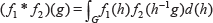
In general, if a manipulator has N segments, then

$f_{\mathrm{1,}\dots \mathrm{,}N}\left(g\right)=(f_1*f_2*\cdots *f_N)\left(g\right)$

(3)

The workspace density f(g) has the following properties.

$f\left(g\right)\ge 0$

(4)

${\displaystyle {\int }_G}f\left(g\right)d\left(g\right)=1$

(5)

So we know workspace density f(g) is a PDF (Probability Density Function).

2.2 Mathematical modeling for the workspace density function

The Fourier transform for rigid-body motions of the plane, SE(2), has been used to compute workspace densities in prior works in [25]. The novel research in the present work is that the workspace densities for planar redundant manipulators can be written in closed-form expression based on the special structure.

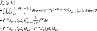
In Fig.1, x₀, y₀ are the base coordinate system. x₁ and y₁ are the coordinate system to describe the pose of the first link. The direction of x₁ axis is along the first link. In the case of a single planar revolute manipulator, we can get ϕ = θ₁ and r = L₁. where L₁ is the length of first link and θ₁ is the angle of first joint. In the polar coordinate system, each point on a plane is determined by a distance r from a fixed point and an angle ϕ from a fixed direction.

The δ function is the Dirac delta function. It is a generalized function on the real number line that is zero everywhere except at zero, with an integral of one over the entire real line. The most important property of the Dirac delta function is

Figure 1.

Kinematic model of a one-link planar robot arm

${\displaystyle {\int }_{R^n}}f\left(t\right)\delta (t-T)dt=f\left(T\right)$

(6)

In one link case, r = L₁ and ϕ = θ₁ = θ, we can use two the Dirac delta functions to express the density function, $f_1(g;L_1)=C_1\frac{\delta (r-L_1)\delta (\phi -\theta )}{r}$ and dt = rdrdϕdθ. Based on (5), the value of workspace function is one when it is integrated on SE(2).

$\begin{array}{ll}\hfill & {\displaystyle {\int }_{SE\left(2\right)}}{f}_1(g;L_1)dg\hfill \\ \hfill & ={\displaystyle {\int }_{r=0}^{\infty }}{\displaystyle {\int }_{\phi =-\pi }^{\pi }}{C}_1\delta (r-L_1)\delta (\phi -\theta )rdrd\phi d\theta =1\hfill \end{array}$

(7)

From (7), we know $C_1=\frac{1}{2\pi }$ . The workspace density function of one link with freely moving revolute joint is expressed as

$f_1(g;L_1)=\frac{1}{2\pi }\frac{\delta (r-L_1)}{r}\delta (\phi -{\theta }_1)$

(8)

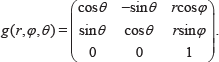
The polar coordinates r and ϕ can be converted to the rectangular coordinates x and y by using the trigonometric functions:

$\{\begin{array}{lll}x\hfill & =\hfill & r\text{cos}\phi \hfill \\ y\hfill & =\hfill & r\text{sin}\phi \hfill \end{array}$

(9)

As a result, the integral of the workspace density function f₁(g; L) over r, θ, and ϕ with respect to the measure d(g) = rdrdθdϕ has a value of unity. Here g(r, θ, ϕ) is the homogeneous transformation matrix with translations parameterized expressed in polar coordinates, where –π≤ϕ, θ≤π.

$g\left(r\mathrm{,}\phi \mathrm{,}\theta \right)=\left(\begin{array}{ccc}\text{cos}\theta & -\text{sin}\theta & r\text{cos}\phi \\ \text{sin}\theta & \text{cos}\theta & r\text{sin}\phi \\ 0& 0& 1\end{array}\right)\mathrm{.}$

(10)

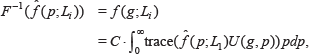
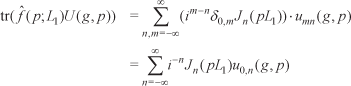
The Fourier transform of a workspace density function, f(g), for SE (2) is defined as

$F\left(f\right)=\widehat{f}\left(p\right)={\displaystyle {\int }_G}f\left(g\right)U\left(g^{-1}\mathrm{,}p\right)d\left(g\right)$

(11)

where U (g⁻¹, p) is a unitary operator that defines the unitary representation of G = SE(2) and d(g) is the natural bi-invariant integration measure for SE(2), and “p” is a frequency-like parameter.

In group theory, the set of all “p” values is called the “unitary dual” of G. The matrix elements of the operator U(g⁻¹, p) are expressed as

$u_{mn}\left(g^{-1}\right(r\mathrm{,}\theta \mathrm{,}\phi ),p)=i^{n-m}{e}^{i[m\theta +(n-m\left)\phi \right]}{J}_{m-n}(pr)$

(12)

Where i is the imaginary number, its property i² = −1. J _v (x) is the v^th order Bessel function. The matrix elements of the Fourier transform can be calculated using the matrix elements of U(g⁻¹, p) as

${\widehat{f}}_{mn}\left(p\right)={\displaystyle {\int }_G}f\left(g\right)u_{mn}\left(g^{-1}\mathrm{,}p\right)d\left(g\right)$

(13)

Substituting (8) and (12) into (13), the result is

$\begin{array}{ll}\hfill & {\widehat{f}}_{mn}(p;L_1)\hfill \\ \hfill & ={\displaystyle {\int }_r}{\displaystyle {\int }_{\phi }}{\displaystyle {\int }_{\theta }}\frac{1}{2\pi }\frac{\delta (r-L_1)}{r}\delta (\phi -\theta )i^{n-m}{e}^{i[m\theta +(n-m\left)\phi \right]}{J}_{m-n}\left(pr\right)rdrd\phi d\theta \hfill \\ \hfill & =i^{n-m}{J}_{m-n}\left(p{L}_1\right){\displaystyle {\int }_{\theta =-\pi }^{\pi }}\frac{1}{2\pi }{e}^{in\theta }d\theta \hfill \\ \hfill & =i^{n-m}{J}_{m-n}\left(p{L}_1\right){\delta }_{\mathrm{0,}n}=i^{n-m}{J}_m\left(p{L}_1\right){\delta }_{\mathrm{0,}n}\hfill \end{array}$

(14)

where δ_0,n is Kronecker delta function that is defined by integer variables m and n as

${\delta }_{m\mathrm{,}n}=(\begin{array}{c}0\text{\hspace{1em}if\hspace{1em}}n\ne m\\ 1\text{\hspace{1em}if\hspace{1em}}n=m\mathrm{.}\end{array}$

(15)

The Convolution Theorem: the Fourier transform of the convolution of two functions is the product of the Fourier transforms of the two functions. This generalizes as

$\begin{array}{ll}F(f_1*f_2)\hfill & ={\displaystyle {\int }_G}\left({\displaystyle {\int }_G}{f}_2\right(g\left)U\right(g^{-1}\mathrm{,}p\left)U\right(h^{-1}\mathrm{,}p)\hspace{0.17em}d(g\left)\right)f_1\left(h\right)\hspace{0.17em}d\left(h\right)\hfill \\ \hfill & =\left({\displaystyle {\int }_G}{f}_2\right(g\left)U\right(g^{-1}\mathrm{,}p)\hspace{0.17em}d(g\left)\right)\left({\displaystyle {\int }_G}{f}_1\right(h\left)U\right(h^{-1}\mathrm{,}p)\hspace{0.17em}d(h\left)\right)\hfill \\ \hfill & =F\left(f_2\right)F\left(f_1\right)={\widehat{f}}_2\left(p\right){\widehat{f}}_1\left(p\right)\hfill \end{array}$

(16)

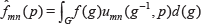
The m–k^th matrix element of Fourier transform matrix f̂²(p; L) is expressed as

$\begin{array}{ll}{\left({\widehat{f}}_2\right(p;L_i\left)\right)}_{mk}\hfill & ={\displaystyle \sum _{n=-\infty }^{\infty }}{\widehat{f}}_{mn}(p;L_1){\widehat{f}}_{nk}(p;L_2)\hfill \\ \hfill & ={\displaystyle \sum _{n=-\infty }^{\infty }}\left(i^{n-m}{J}_m\right(p{L}_1\left){\delta }_{\mathrm{0,}n}\right)\cdot \left(i^{k-n}{J}_n\right(p{L}_2\left){\delta }_{\mathrm{0,}k}\right)\hfill \\ \hfill & =i^{k-m}{J}_m\left(p{L}_1\right)J_0\left(p{L}_2\right){\delta }_{\mathrm{0,}k}=J_0\left(p{L}_2\right){\widehat{f}}_{mk}(p;L_1)\hfill \end{array}$

(17)

Based on the above derivation, it is easy to find the elements of the Fourier transform matrix for the N-link is

${\left({\widehat{f}}_N\right(p;L_i\left)\right)}_{mn}={\displaystyle \prod _{i=2}^N}{J}_0\left(p{L}_i\right){\widehat{f}}_{mn}(p;L_1)$

(18)

To reconstruct f(g), we can invert f̂ _mn (p; L₁) using the invert Fourier transform as follows,

$\begin{array}{ll}{F}^{-1}\left(\widehat{f}\right(p;L_i\left)\right)\hfill & =f(g;L_i)\hfill \\ \hfill & =C\cdot {\displaystyle {\int }_0^{\infty }}\text{trace}\left(\widehat{f}\right(p;L_1\left)U\right(g\mathrm{,}p\left)\right)pdp\mathrm{,}\hfill \end{array}$

(19)

where $C=\frac{1}{{\left(2\pi \right)}^2}$ . The elements of the unitary operator U(g, p) are expressed as

$u_{mn}\left(g\right(r\mathrm{,}\theta \mathrm{,}\phi ),p)=i^{n-m}{e}^{-i[n\theta +(m-n\left)\phi \right]}{J}_{n-m}(pr)$

(20)

The workspace density of N-link robotic manipulator is denoted as f_N (g; L _i ,) which is reconstructed by (19).

$\begin{array}{ll}{f}_N(g;L_i)\hfill & =(f*f*\cdots *f)(g;L_i)\hfill \\ \hfill & =C\cdot {\displaystyle {\int }_0^{\infty }}{\displaystyle \prod _{i=2}^N}{J}_0(p{L}_i)\text{tr}(\widehat{f}(p;L_1)U(g\mathrm{,}p))pdp\hfill \end{array}$

(21)

where

$\begin{array}{ll}\text{tr}(\widehat{f}(p;L_1)U(g\mathrm{,}p))\hfill & ={\displaystyle \sum _{n\mathrm{,}m=-\infty }^{\infty }}(i^{m-n}{\delta }_{\mathrm{0,}m}{J}_n(p{L}_1))\cdot u_{mn}(g\mathrm{,}p)\hfill \\ \hfill & ={\displaystyle \sum _{n=-\infty }^{\infty }}{i}^{-n}{J}_n(p{L}_1)u_{\mathrm{0,}n}(g\mathrm{,}p)\hfill \end{array}$

2.3 Numerical computation of workspace density

A three-link planar revolute robot arm is shown in Fig.2. Three link lengths specify the geometry of the planar robot, and three angles specify its conformation. Let L₁, L₂ and L₃ denote the lengths of the three links and θ₁, θ₂ and θ₃ denote the joint angles between the links. The definition for the joint angle θ _i is measured counter clockwise from link i −1 to link i. The position and orientation of the end-effector are presented in the Cartesian coordinate system as

$(\begin{array}{c}x=L_1\text{cos}{\theta }_1+L_2\text{cos}({\theta }_1+{\theta }_2)+L_3\text{cos}({\theta }_1+{\theta }_2+{\theta }_3)\\ y=L_1\text{sin}{\theta }_1+L_2\text{sin}({\theta }_1+{\theta }_2)+L_3\text{sin}({\theta }_1+{\theta }_2+{\theta }_3)\\ \theta ={\theta }_1+{\theta }_2+{\theta }_3\\ \end{array}$

(22)

Figure 2.

The kinematic model of a three-link planar robot arm

We can get sampling-based workspace density of three-link planar manipulators based on (22) by following steps:

1. Initialization. Set L₁ = L₂ = L₃ = 1.25 and randomly generator 1000 values of each θ _i in the range of [–π, π].

2. Compute the pose of end effector (x, y, θ) by (20).

3. According to the different scope of θ, $\theta ,[\pi \mathrm{,}-\frac{\pi }{2}),[-\frac{\pi }{2}\mathrm{,0}),\left[\mathrm{0,}\frac{\pi }{2}\right),\left[\frac{\pi }{2}\mathrm{,}\pi \right]$ , we divide results into four groups.

4. We plot the histogram of points based on (1) the definition of workspace density of each group.

In the left column (subfigures (a), (c), (e), (g)) of Fig. 3 are the density obtained from sampling.

In the right column (subfigures (b), (d), (f), (h) show the discrete workspace density and the corresponding density of this manipulator with three links generated from the Fourier method based on (21). The number of links N = 3 and the length of links L₁ = L₂ = L₃ = 1.25. The workspace density of θ ε [a,b] is computed by integrating f₃(g; L₃) on [a,b]. The function of workspace density of three-link planar manipulator is

$\begin{array}{ll}\hfill & {\displaystyle {\int }_a^b}{f}_3(g;L_3)d\theta \hfill \\ \hfill & =\frac{1}{{(2\pi )}^2}{\displaystyle {\int }_a^b}{\displaystyle {\int }_0^{\infty }}{\displaystyle \prod _{i=2}^3}J(p{L}_i){\displaystyle \sum _{n=-\infty }^{\infty }}{J}_n(p{L}_1)e^{-i[n\theta -n\phi ]}{J}_n(pr)pdpd\theta \hfill \\ \hfill & =-\frac{1}{in{(2\pi )}^2}{\displaystyle {\int }_0^{\infty }}{\displaystyle \prod _{i=2}^3}J(p{L}_i){\displaystyle \sum _{n=-\infty }^{\infty }}{J}_n(p{L}_1)e^{in\phi }{e}^{-in(b-a)}{J}_n(pr)pdp\hfill \\ \hfill & =-\frac{1}{in{(2\pi )}^2}{\displaystyle {\int }_0^{\infty }}{\displaystyle \prod _{i=2}^3}J(p{L}_i){\displaystyle \sum _{n=-\infty }^{\infty }}{J}_n(p{L}_1)e^{in(\phi -b+a)}{J}_n(pr)pdp\hfill \end{array}$

(23)

Figure 3.

Comparison of the sample-based workspace density with the corresponding density of this manipulator with three links generated from the fourier transform

The workspace W is divided into many small boxes. The center of small box (x_i, y_i) is changed to (r _i , ϕ _i ) based on (9) as the input of function (23). All the results are plotted in histograms. Fig.3 (a) and 3(b) compare the workspace density of $\theta \in [-\pi \mathrm{,}-\frac{\pi }{2})$ . In Fig. 3 (c) and 3(d), $\theta \in [-\frac{\pi }{2}\mathrm{,0})$ . In Fig.3 (e) and 3(f), $\theta \in \left[\mathrm{0,}\frac{\pi }{2}\right)$ . In Fig. 3 (g) and 3(h), $\theta \in \left[\frac{\pi }{2}\mathrm{,}\pi \right]$ . Fig.3 compares the discrete workspace density with the corresponding density of this manipulator with three modules generated from the SE(2) Fourier transform. As can be seen, the shape and size of workspace of three-link planar manipulators are similar. The maximal values of density appear in the same areas. Comparison results show the workspace density function can effectively describe the workspace of the planar redundant manipulator.

3. The algorithm for obstacle avoidance in path planning

We solve the obstacle avoidance problem based on the workspace density using our Fourier-based approach. This approach is similar to the method in [28], which presented an inverse kinematics algorithm of binary manipulators with many actuators. The criterion of our approach is to select joint angles so as to obtain the maximum workspace density near the aim point to fix configuration of the manipulator shown in Fig.4. In Fig.4, the number of the links N and the length of the links L_i are given on the start step. g_aim denotes the homogenous transformation of target pose. All possible states of one joint are denoted by manipulator workspace, obstacle avoidance, convolution theorem, path planning with their ranges computed by the collision checks algorithm. The homogenous transformation of k^th link is denoted by g_k, where k ε {1,2, ···, N}. For the k^th link, g_k maximizes the workspace density f_N–k ((g₁ g₂ ··· g_i)⁻¹ ga_aim). Then we fix the homogenous transformation g_k for the k^th link. Then we compute the manipulator one link at a time. In all possible states, we search for g_k+1 that can obtain the highest density f_N–k−1((g₁ g₂ ··· g_k g_k+1)⁻¹ g_aim). If g_k+1 is such a state, we configure the (k + 1) ^th module to g_k+1. This program is performed by sequentially maximizing density from the first to (N − 1) ^th link. At the last step i = N, we compute the minimum distance between the pose of N ^th link and the goal pose, and fix g_N.

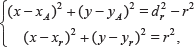
In steps of this path planning method, obstacle checking is an important step for this algorithm. For the different shape of obstacles, we make externally tangent circle for them. Computing the distance d_r between the center of externally tangent circle and the end of each link to do the obstacle checks before find g_ii for each link. From Fig.5, we know that if dr > r + L the manipulator could not encounter obstacles. Then we can choose g_i from free range. If dr < r + L, the manipulator will encounter obstacles. Then we can compute g_ii by a limited range that depends on the pose of obstacle, where r is the radius of obstacle and L is the length of each link.

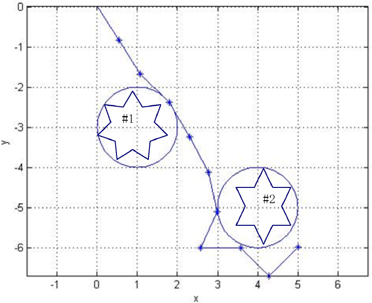
We can compute the limited angle of joint for the link using geometric method based on the properties of vector. In Fig. 6, the new range of angle is [[–π, π] – [θ₁, θ₂]].

Based on the geometric relationship in Fig.6, we have

$(\begin{array}{c}{(x-x_A)}^2+{(y-y_A)}^2=d_r^2-r^2\\ {(x-x_r)}^2+{(y-y_r)}^2=r^2\mathrm{,}\end{array}$

(24)

where (x_A, y_A) denotes the position of points A and (x_r, y_r) denotes the position of the center for the externally tangent circle. A and B are intersections of the circle (center(x_r, y_r), radius = r) and circle (center(x_A, y_A), radius = d _r ² – r². The position of B(x_B, y_B) and C(x_C, y_C) are the solutions of (24).

Figure 4.

Flowchart for the obstacle avoidance of inverse kinematics

The vectors of $\overline{OA}$ and $\overline{AC}$ are computed by the position of points O, A, B and C.

$\{\begin{array}{l}\overline{OA}=(x_A-x_O\mathrm{,}{y}_A-y_O)\hfill \\ \overline{AB}=(x_B-x_A\mathrm{,}{y}_B-y_A)\hfill \\ \overline{AC}=(x_C-x_A\mathrm{,}{y}_C-y_A)\hfill \end{array}$

(25)

Figure 5.

Kinematic model of a three-link planar robot arm

Figure 6.

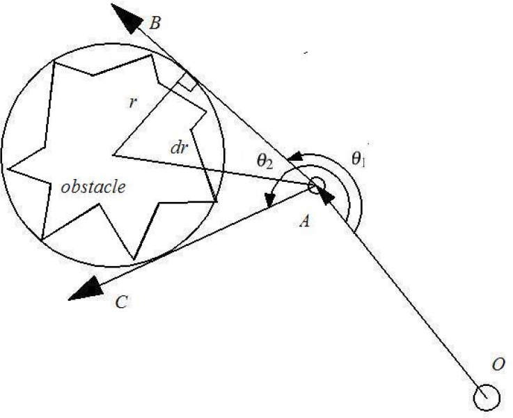
Geometric model of obstacle check

Generally speaking, if the direction of angle is counterclockwise, we set the value of angle to positive. On the contrary, if the direction of angle is clockwise, we set the value of angle to negative. Using the properties of vectors, we have θ₁ and θ₂ as follows

${\theta }_1=D_1\cdot \text{arccos}\left(\frac{\overline{\text{OA}}\cdot \overline{\text{AB}}}{\text{|OA|}\cdot \text{|AB|}}\right)$

(26)

and

${\theta }_2=D_2\cdot \text{arccos}\left(\frac{\overline{\text{OA}}\cdot \overline{\text{AC}}}{\text{|OA|}\cdot \text{|AC|}}\right)\mathrm{,}$

(27)

where D₁ and D₂ denote the direction of θ₁ and θ₂. The direction of angle can be obtained by computing the cross product of vectors which compose the angle. D₁, the direction of θ₁, is computed by (28). D₂ is computed by using the same method. In the special case, when cross product of two vectors equals zero, the two vectors are coincident, and the angle between the two vectors equals zero..

$\{\begin{array}{l}\text{if\hspace{1em}}\overline{OA}\times \overline{AB}\ge 0D_1=1\hfill \\ \text{if\hspace{1em}}\overline{OA}\times \overline{AB}=0D_1=0\hfill \\ \text{if\hspace{1em}}\overline{OA}\times \overline{AB}\le 0D_1=-1\hfill \end{array}$

(28)

4. Simulations of obstacle avoidance path planning

The manipulators with 10 links is used to illustrate the obstacle avoidance path planning approach. The length of each link L =1. We set the pose of aim point $\left(x_{aim}\mathrm{,}{y}_{aim}\mathrm{,}{\theta }_{aim}\right)=(\mathrm{5,}-\mathrm{6,}\frac{\pi }{4})$ . The position of externally tangent circle center for #1 obstacle is (1,-2) and the radius of circle is 0.6. The position of externally tangent circle center for #2 obstacle is (2,-4) and the radius of circle is 0.5. The obstacle avoidance path planning algorithm in Section 3 is now demonstrated with the workspace density from (21). The simulation result is shown in Fig.7. The segmented lines stand for links of robotic manipulators and display the corresponding configurations of the manipulator.

Figure 7.

A simulation result of the inverse kinematics method

In Fig.8, the target pose is $\left(x_{aim}\mathrm{,}{y}_{aim}\mathrm{,}{\theta }_{aim}\right)=(-\mathrm{5,5,}\frac{\pi }{3})$ . The position of externally tangent circle center for #1 obstacle is (−2,1) and the radius of circle is 0.6. The position of externally tangent circle center for #2 obstacle is (−4,3) and the radius of circle is 0.7.

In Fig.9, the target pose is $\left(x_{aim}\mathrm{,}{y}_{aim}\mathrm{,}{\theta }_{aim}\right)=(\mathrm{5,}-\mathrm{6,}\frac{\pi }{3})$ . The position of externally tangent circle center for #1 obstacle is (1,-3) and the radius of circle is 1. The position of externally tangent circle center for #2 obstacle is (4,-5) and the radius of circle is 1.

Figure 8.

A simulation result of the inverse kinematics method

Figure 9.

A simulation result of the inverse kinematics method

From the simulation results, we can see that the inverse kinematics algorithm ensures that the base manipulators are close to the target in an obstacle environment. Then the end manipulators have more flexibility when they close to the target. The algorithm of inverse kinematics also can find a path in the narrow spaces between obstacles from the result of the simulation in Fig.9.

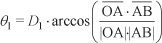
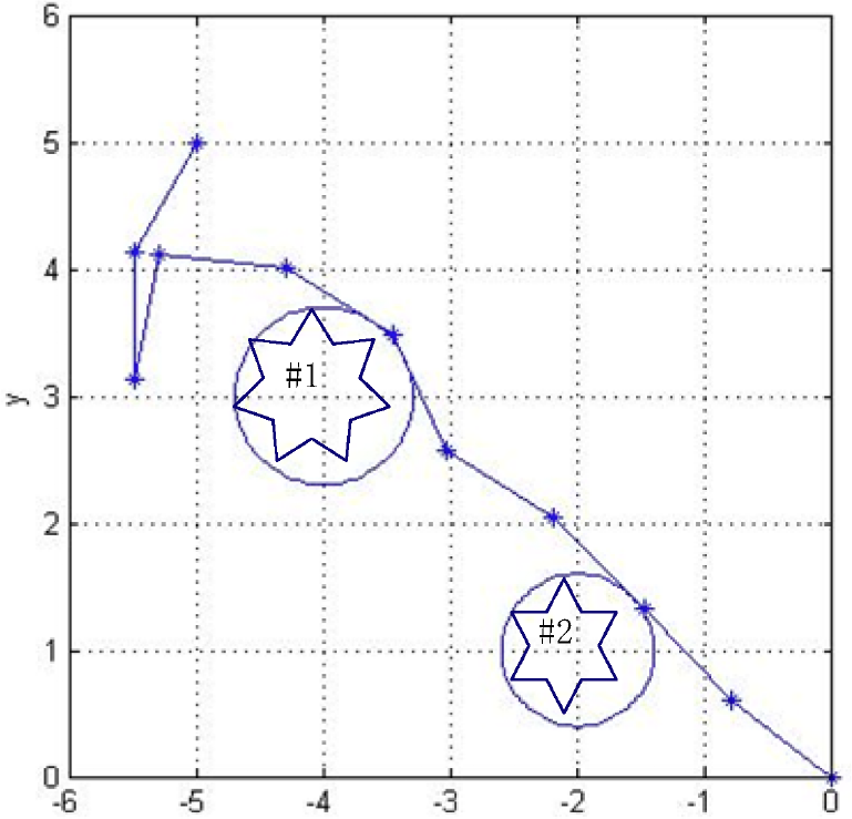
To illustrate the efficacy of the sample-based workspace density approach, we solve the path planning problem using this approach. Consider generating a path from starting pose $\left(\mathrm{1.5,5,}\frac{\pi }{3}\right)$ to ending pose $\left(\mathrm{4.5,5,}\frac{\pi }{3}\right)$ in the free workspace. The position of externally tangent circle center of #1 obstacle is (3,5) and the radius of circle is 0.5. The path is divided into 6 steps. Each step is solved by the algorithm of inverse kinematics. On the right side of Fig.10 is the simulation result of the method proposed in this paper, the joint of each link changes a slight angle at each step that ensure minimum energy consumed between steps.

The same problem is solved by rapidly exploring random trees (RRT)[29]. The left side of Fig.10 shows the simulation result of the RRT approach. The red path is the final result chosen as the path of manipulators.

Figure 10.

Comparison of simulation results of the Sample-Based Workspace Density method with the RRT method of the obstacle avoidance path planning

Comparison with the simulation results, the following conclusion can be obtained:

1. The RRT algorithm needs to provide the initial state and the end state based on the inverse kinematics. The algorithm based on the workspace density function only need to provide the starting pose and ending pose. The algorithm contains the method of solving inverse kinematics.

2. The result of the RRT depends on initial conditions. The problem can not be solved based on some initial conditions every time. The algorithm based on the workspace density function can find the result in the free workspace which does not depend on the initial conditions.

3. The result of the RRT has strong randomness. The results are different with the same initial conditions. The result of RRT cannot be guaranteed to be the good result. The result of algorithm based on the workspace density function is the same with the same conditions. The path is smooth and short.

5. Conclusion

We efficiently generate the workspace density of the planar redundant manipulators using a combination of the concept of the Fourier transform for the group of rigid-body motions of the plane, the resulting convolution theorem, and the particular form of the workspace density of a single link in a planar redundant manipulator. The significance of this approach is that it selects a solution from among a very large discrete set using workspace density as an evaluation criterion to solve the obstacle avoidance path planning problem.