Kinodynamic Motion Planning for Autonomous Vehicles

Abstract

This article proposes a computationally effective motion planning algorithm for autonomous ground vehicles operating in a semi-structured environment with a mission specified by waypoints, corridor widths and obstacles. The algorithm switches between two kinds of planners, (i) static planners and (ii) moving obstacle avoidance manoeuvre planners, depending on the mobility of any detected obstacles. While the first is broken down into a path planner and a controller, the second generates a sequence of controls without global path planning. Each subsystem is implemented as follows. The path planner produces an optimal piecewise linear path by applying a variant of cell decomposition and dynamic programming. The piecewise linear path is smoothed by Bézier curves such that the maximum curvatures of the curves are minimized. The controller calculates the highest allowable velocity profile along the path, consistent with the limits on both tangential and radial acceleration and the steering command for the vehicle to track the trajectory using a pure pursuit method. The moving obstacle avoidance manoeuvre produces a sequence of time-optimal local velocities, by minimizing the cost as determined by the safety of the current velocity against obstacles in the velocity obstacle paradigm and the deviation of the current velocity relative to the desired velocity, to satisfy the waypoint constraint. The algorithms are shown to be robust and computationally efficient, and to demonstrate a viable methodology for autonomous vehicle control in the presence of unknown obstacles.

1. Introduction

Exploitation of the versatility of autonomous vehicles for academic, industrial and military applications will have a profound effect on our collective future. Unmanned ground vehicles (UGVs), when integrated into our vehicle-centric lives, have some very promising applications. One such application is demonstrated by vehicles designed for the Defence Advanced Research Projects Agency Urban Challenge (DUC) [1, 2].

1.1. Motivations

This work is motivated by the applications of UGVs operating on highways or racecourses. For such applications of UGVs to be viable, it is imperative that a safe motion path should be generated in real-time. To achieve this goal, the autonomous motion planning system should handle not only global path planning but also local obstacle avoidance. The development of wireless technology and a ubiquitous data/computing environment enables the UGV to easily obtain the required information for global path planning, such as GPS coordinates and/or road information, at any location and at any time. As the vehicle follows this globally planned path based on high-level information, it is necessary to detect and safely miss local obstacles, such as pedestrians, debris or other cars on the road. In the real world, the local environment of the vehicle is unknown and dynamically changing due to limited vehicle sensor range, making it critical for obstacle avoidance to be performed within very tight time bounds. This research proposes a computationally efficient motion planing algorithm for the UGV to operate in this type of cluttered environment.

1.2. Related Works

A significant amount of work has been dedicated to the problem of motion planning over recent decades.

Despite many external differences, the various path planning algorithms can be formulated into queries as graph searches, in which discrete robot states (vertices) are connected by motion segments (edges). Adequate techniques for constructing search graphs are selected depending on the type of map: (i) feature-based and (ii) location-based. The feature-based maps specify the shapes and locations of objects in the environment. While feature representation is compact and makes it easier to adjust the position of an object, it may be very difficult to update unknown environments in real-time due to the computational complexity involved in recognizing features. Visibility graph-type [3] approaches produce the shortest Euclidean paths in the map with polygonal obstacles. The method has been widely used to implement path planners for mobile robots [3, 4]. The Voronoi diagram approach, introduced by Ó'Dúnlaing et al. [5], provides a retracted configuration space that maximizes the clearance between the robot and obstacles. Sahraei et al. [6] and Choi et al. [7] have presented a motion planning algorithm for omnidirectional vehicles by applying the Voronoi diagram method in combination with Dijkstra's shortest path search algorithm.

Another approach, called cell decomposition, consists of decomposing the vehicle's free space (C_free) into a collection of non-overlapping cells and constructing the connectivity graph between cells. The concept of cell decomposition has been extended into a large number of path planning techniques. Chatila [8] applied an exact decomposition of the workspace into convex cells for motion planning with incomplete knowledge for a mobile robot. Avnaim et al. proposed a variant of cell decomposition to plan the path of the vehicle among polygonal obstacles by decomposing C_free's boundary rather than C_free. Lingelbach [9] combined cell composition with probabilistic sampling to obtain a method called Probabilistic Cell Decomposition.

Another type of map is location-based. A classical map representation known as occupancy grid map is location-based. The map assigns to each coordinate a binary value which indicates whether or not a location is occupied with an object. Occupancy grid maps are an efficient means for quickly updating any unknown local terrain surrounding the robot, but they tend to pay the price of large memory requirements. While conventional grid-based path planners use discrete state transitions connecting centre points of grid cells so that the robot's motion is constrained to a small set of headings, Ferguson and Stentz used linear interpolation to calculate accurate path cost estimates for arbitrary positions within each grid cell in order to produce paths with a range of continuous headings [10]. Pivtoraiko and Kelly efficiently converted occupancy grid maps into graph representations for differentially constrained motion queries [11]. The search graphs were constructed by connecting a finite set of feasible motion segments between repeating pairs of discrete robot states.

Performing search algorithms on the resulting graphs may produce free paths. A^*, proposed by Hart [12], is one of the most widely used search algorithms in path planning. Most of the DUC teams [1, 2] have demonstrated robust path generation by adapting A^* or its variants, such as [13, 14]. While A^* is a deterministic search, rapidly-exploring random trees (RRT), introduced by LaValle and Kuffner [15], is one of the most popular probabilistic search algorithms. Randomized approaches are thought to be incomplete but nonetheless exhibit effectiveness in solving many challenging problems, ranging from autonomous navigation [16] to robotic manipulation [17]. When it is possible to give the robot maps in advance, the search performance can be further improved by applying dynamic programming (DP) which pre-calculates and reuses the shortest path information on the maps provided. Suh [18] placed a sequence of dividing lines to partition a free space (C_free) and discretized the lines into a finite number of points. Afterwards, the optimal path was constructed by each point determined using DP on each line. Barraquand [19] discussed potential-based DP applied to various submanifolds of the configuration space. Flint [20] proposed a model of a cooperative path planning system for multiple autonomous vehicles within the framework of a DP decision process.

Even though many path search algorithms [10, 13, 14] provide computationally efficient methods in discrete state spaces, the resulting paths tend not to be smooth (piecewise linear) and, hence, do not indicate the kinematic feasibility of the robot. It is necessary to smooth the paths. The B-spline is a well-known parametric curve for smoothing a linear path. The continuity of the derivatives of a given order at the joint nodes between elementary segments leads to smoothness. Many researchers have come up with B-spline-based path planning methods. However, when spline methods are applied to a piecewise linear path, there is no guarantee of a collision-free path in a cluttered environment [21]. Since B-splines exhibit a high degree of dependency between their elementary segments, it is difficult to find an efficient way to adjust the path such that it misses a colliding obstacle. Most approaches proposed so far manually move the control points until the path misses the obstacle [4, 21]. To avoid this inefficiency, Bézier curves have been used for path smoothing. Yang and Sukkarieh et al. [21] used cubic Bézier spiral curves to produce obstacle avoiding curvature continuous paths. Choi et al. [22] produced curvature continuous piecewise Bézier curve paths by minimizing the cost determined by arc length and curvature under a boundary constraint in C_free.

One of the most challenging problems in autonomous motion planning may be moving obstacle avoidance. Fiorini [23] proposed the concept of a velocity obstacle (VO), which is the set of velocities that leads to a collision with an obstacle at some moment in time. Variations of the concept have been discussed. For example, the nonlinear velocity obstacle (NLVO) generalizes (VO) to obstacles moving along arbitrary trajectories [24]. The reciprocal velocity obstacle (RVO) was proposed for multi-agent navigation. RVO takes into account the reactive behaviour of the other agents to guarantee collision- and oscillation-free motions for each agent [25]. Velocity obstacles remain an ongoing area of robot navigation research.

1.3. Problem Statement

The problem we address here is formulated as follows. Consider the motion planning problem of an autonomous ground vehicle to operate in the route in-bounds area specified by a sequence of waypoints W = {w₁, …, w _N } and corridor widths between two successive waypoints L = {l₁,…, l_N-1}, and filled with unknown obstacles O = {o₁,…, o _M }, as shown in Figure 1. We assume that the vehicle is given the road information W, L in advance. This may be legitimate in real world applications equipped with mobile computing systems; however, the local obstacles O surrounding a vehicle are unknown and dynamically changing in the real world.

Figure 1.

A mission route in-bounds area specified by five waypoints and four corridor widths and containing three obstacles

The motion of the vehicle is modelled by z = (x, y,ψ) ^T , the state, and u = (v,k) ^T , the control vector, where (x,y) and ψ represent the position and orientation, and v and k are the longitudinal velocity and the instantaneous curvature of the vehicle (Figure 2). Then, the kinematic equation of the vehicle is given by:

Figure 2.

Schematic drawing of dynamic model of vehicle motion

$$\dot{x}=v\cos \psi ,\dot{y}=v\sin \psi ,\dot{\psi }=v\kappa \mathrm{.}$$

(1)

The control signal is bounded due to the limits on the tangential and radial acceleration, a_tMax and a_rMax:

$$\begin{array}{l}-a_{tMax}\le \frac{dv}{dt}\le a_{tMax},-\frac{a_{rMax}}{v^2}\le \kappa \le \frac{a_{rMax}}{v^2}\mathrm{.}\hfill \end{array}$$

(2)

1.4. System Architecture

Our goal is to develop and implement a computationally efficient algorithm for the real-time navigation of a vehicle operating in the mission route specified by W, L, O. Figure 3 shows our autonomous navigation system architecture, which exploits two kinds of motion planners - namely, static planners and moving obstacle avoidance manoeuvre planners - in a mutually exclusive way, depending on the mobilities of the detected obstacles.

Figure 3.

The autonomous navigation system architecture

When the vehicle operates in a stationary workspace, a classic motion planner which combines a path planner and a controller will be selected. Given the free configuration space C_free determined by W, L, O, an initial state z _init and a goal state z _goal of the vehicle, the path planner produces a free path Γ:

$$\text{Γ}:[\mathrm{0,1}]\to {\mathcal{C}}_{free},$$

subject to the kinodynamic constraints (1) and (2) and the boundary constraint:

$$\text{Γ}(0)=z_{init},\text{\hspace{1em}Γ}(1)=z_{goal}\mathrm{.}$$

(3)

(Section 2 presents the path planning algorithm in detail.)

The basic task of the controller is to generate a control command u to be exerted by the actuator such that the vehicle follows the path Γ. Typically, the transformation is divided into two steps. The first step, called trajectory generation, computes the time dependence of the continuous sequence of states by determining velocity profile along γ. Prior to motion execution, the output is fed into the next step as the desired trajectory z _d (t). The second step, called trajectory tracking, computes the control command from the deviation of the current state z _s relative to z _d , such that the vehicle's actuator performs the desired motion. Iteratively, z _s is fed back into the controller to compute u, as illustrated in Figure 3. (Section 3 details the implementation of the controller.)

While the static obstacle avoidance manoeuvre has the advantage of breaking down the motion planning problem into clearly defined sub-problems, it may be inefficient when the vehicle operates in a dynamic workspace among mobile obstacles, and when the task to be accomplished is within tight time bounds. In such cases, it is more efficient to incorporate the dynamic constraint of the vehicle during motion planning to produce time-optimal motions for execution, as detailed in Section 4

1.5. Contributions

This article demonstrates significant contributions in kinodynamic motion planning for UGVs operating in a semi-structured environment.

• To deal with the path planning problem addressed in Section 1.3, we propose an efficient algorithm which works better than the widely-known A^* or RRT as applied to occupancy grid maps, for the following reasons: (i) Classical A^* and RRT incrementally construct search graphs by using discrete motion primitives. While these methods have been proven to be efficient for many path planning problems in unknown environments, they have the drawback of requiring a relatively large number of variables to convert grid maps into graphs. Since the complexity of a search increases as the size of the graph increases, incremental methods may be inadequate for application to large environments, such as MR, which we address. On the other hand, our method converts a feature-based map W, L into a more compact graph representation by applying cell decomposition (CD) and, hence, reducing complexity. The implementation of CD is enabled by the assumption that the vehicle is given feature-based maps in advance. (ii) In the context of re-planning, algorithms such as A^* and RRT compute the shortest paths from scratch. On the other hand, our algorithm applies dynamic programming (DP) for offline computation and to reuse the globally shortest path information, thereby reducing the computation time used for re-planning. D^* – Lite [13], a variant of A^*, updates the knowledge of the local environment and reuses information from previous searches to find solutions. However, the size of the updated information and the degree of complexity of re-planning for grid maps remain greater than those of our method. The uniqueness of our method is to use cutting edges determined by dividing parameters on boundary of the C_free so that a relatively large environment is represented by a few variables. Every time the vehicle detects obstacles, C_free is efficiently re-decomposed using the edges. Incorporating DP with the graph efficiently generates smooth and safe paths. (Section 2.1–2.2.)

• For the task of path smoothing with an obstacle avoidance constraint, many of the approaches proposed so far manually move the control points of splines until the path misses the obstacle [4, 21]. Meanwhile, this paper provides analytic solutions to minimize the maximum curvature of the smoothing curves while satisfying the constraint. (Section 2.3)

• The analysis on the constrained curvature minmax problem is effectively incorporated to generate the highest admissible velocity profile along reference paths, consistent with the vehicle's dynamic constraint. (Section 3)

• This paper also proposes a velocity obstacle-based (VO-based) manoeuvre for real-time moving obstacle avoidance. A common property of VO-based algorithms is that the velocity of the vehicle should be selected from or toward the outside of VO regions to avoid obstacles. The algorithm proposed here calculates a set of safe velocities in discrete time by minimizing the cost expressed in terms of expected collision times and the safety of the current velocity against obstacles in the VO paradigm. While previous work has generated safe motions in free space, it is demonstrated that the algorithm is applicable to the avoidance of moving obstacles with waypoints and corridor constraints. (Section 4)

2. Path Planning

This section proposes a computationally efficient path planning algorithm to satisfy the mission route (MR) constraint.

The algorithm uses cell decomposition to convert MR into a graph composed of a finite set of points cutting the MR (in Section 2.1). Next, dynamic programming (DP) is applied to search the sequence of points constructing the shortest path (in Section 2.2). DP allows the shortest path information on the graph to be pre-calculated and reused and, thereby, reduces the re-planning time. Since the output of the path searching method is a piecewise linear path which violates the nonholonomic nature of the vehicle, it is necessary to smooth the path. We present an efficient path smoothing method based on Bézier curves (in Section 2.3). Finally, we present the re-planning process as knowledge of local space changes due to newly detected obstacles (in Section 2.4). The set of cutting points is used to re-decompose C_free. Incorporating DP with the modified graph generates smooth and safe paths within tight time bounds.

2.1. Route Decomposition

The constrained in-bounds area S (Figure 1) is defined as of the DARPA Grand Challenge 2005. According to the challenge's rule, S can be represented as the union of the route segments denoted by G_i, i = 1, …, N − 1. The i-th segment G_i is constructed by inflating w _i w_i+1 by l_i, as shown in Figure 4(a). Let us introduce additional notation by referring to the figure. The inside (or outside) boundary line segment of G_i is denoted by a _i ⁱⁿ b _i ⁱⁿ (or a _i ^out b _i ^out ). The pivot point is the intersection point of the two successive inside boundary line segments.

Figure 4.

An example of the route decomposition

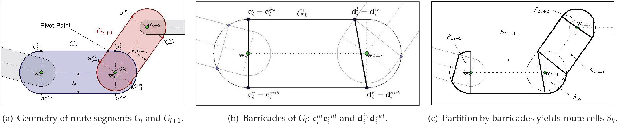
Note that there is an intersection area of two successive route segments. This is a poor structure for the proposed path planning algorithm presented in Section 2.2, because the algorithm applies dynamic programming. That is, the path planning problem is broken down into sub-problems to compute the points constructing the optimal path in each segment comprising S. Hence, it is desirable to decompose S into a finite number of non-overlapping and non-empty cells, S_j, j = 1, …, 2N − 3. To avoid confusion with the route segment G_i, we refer to S_j as the route cell. The cell is constructed by cutting each route segment G_i with two line segments c _i ⁱⁿ c _i ^out and d _i ⁱⁿ d _i ^out , called the barricades, as shown in Figure 4(b). Both of the line segments cut the rectangle a _i ⁱⁿ b _i ⁱⁿ b _i ^out a _i ^out across the centre line w _i w_i+1. None of the four points lie inside any route segment. Under the constraints, c _i ⁱⁿ c _i ^out and d _i ⁱⁿ d _i ^out are determined such that the area of the polygon c _i ⁱⁿ c _i ^out d _i ^out d _i ⁱⁿ is maximized.

Figure 4(c) shows the resulting partition of S. S_2i-1 called the straight cell, is bounded by the polygon c _i ⁱⁿ c _i ^out d _i ^out d _i ⁱⁿ at the straight area between w _i and w_i+1. S_2i, called the corner cell, is bounded by the least restrictive boundary of d _i ⁱⁿ d _i ^out , c_i+1 ⁱⁿ c_i+1 ^out , and the larger circular arcs b _i ^out w_i+1 b _i ⁱⁿ and a_i+1 ⁱⁿ w_i+1 a_i+1 ^out at the corner area around w_i+1. As a result, the total number of cells in the route is 2N − 3.

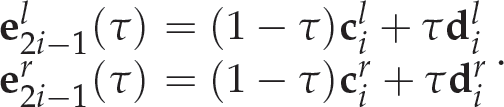
Consider the edge that connects one point on the left outer boundary and the other on the right of the route cell, as shown in Figure 5. Since the edge cuts S across the centre line that connects two successive waypoints, it is called the cutting edge, and the reference path must cross over the edge to satisfy the corridor constraint. Let e _k ^l and e ^r _k denote the two points to construct the cutting edge, on the left and on the right outer boundaries of S_k, respectively. The points are generated by dividing each boundary with the same ratio, τ ∊ (0,1). Given τ, the points are denoted as e _k ^l (τ) and e _k ^r (τ). Figure 5 shows the geometry of the points for each type of cell. Since the left and the right outer boundaries of the straight cell S_2i-1 are line segments, c _i ^l d _i ^l and c _i ^r d _i ^r (Figure 5(b)), its cutting edge points for τ are represented as:

Figure 5.

Definition of cutting edges depending on types of cells

$$\begin{array}{ll}{e}_{2i-1}^l(\tau )\hfill & =(1-\tau )c_i^l+\tau d_i^l\hfill \\ e_{2i-1}^r(\tau )\hfill & =(1-\tau )c_i^r+\tau d_i^r\hfill \end{array}\mathrm{.}$$

(4)

Unlike the straight cell, the left and the right outer boundaries of the corner cell S_2i are a circular arc, $c_{i+1}^l{\stackrel{⌢}{\mathrm{w}}}_{i+1}{d}_i^l$ and $d_i^r{\stackrel{⌢}{\mathrm{w}}}_{i+1}{c}_{i+1}^r$ . To represent the edge points, let ζ _i ^l and ζ _i ^r denote the headings of the vectors d _i ^l − w_i+1 and d _i ^r − w_i+1. Let ϕ _i ^l 0 and ϕ _i ^r > 0 denote the central angles of $c_{i+1}^l{\stackrel{⌢}{\mathrm{w}}}_{i+1}{d}_i^l$ and $d_i^r{\stackrel{⌢}{\mathrm{w}}}_{i+1}{c}_{i+1}^r$ (Figure 5(a)). Also, let T(θ) denote the unit vector corresponding to the angle θ. The edge points can be represented in terms of the notations:

$$\begin{array}{ll}\hfill & e_{2i}^l(\tau )=w_{i+1}+\parallel d_i^l-w_{i+1}\parallel T({\zeta }_i^l-\tau {\varphi }_i^l),\hfill \\ \hfill & e_{2i}^r(\tau )=w_{i+1}+\parallel d_i^r-w_{i+1}\parallel T({\zeta }_i^r+\tau {\varphi }_i^r)\mathrm{.}\hfill \end{array}$$

(5)

Note that when the pivot point exists, e_2i ⁱⁿ (τ) is set to the point for all τ (Figure 5(c)).

It is straightforward that, as τ varies from 0 to 1, the cutting edge e _k ^l (τ)e ^r _k (τ) sweeps the containing cell S_k. So, every point inside of S, denoted by r, can be considered to be on the cutting edge e ^l _k (τ)e ^r _k (τ) specified by the three-tuple (k, τ, ζ), in which k is the index of the containing route cell and τ and ζ are the longitudinal and lateral ratios of the point over the cell, such that:

$$\begin{array}{ll}r=\hfill & \varsigma e_k^r(\tau )+(1-\varsigma )e_k^l(\tau ),\hfill \\ \hfill & k=1,\dots ,2N-3,\tau ∊[\mathrm{0,1}],\varsigma ∊[\mathrm{0,1}]\mathrm{.}\hfill \end{array}$$

(6)

2.2. Primitive Path Search

The next step is to generate the piecewise linear path, namely the primitive path (PP), on the decomposed space.

Let $ℛ=(r_1,r_2,\dots ,r_{n_r})$ denote the sequence of nodes to construct the PP. The first point and the last point must be set equal to the initial position s and goal position t:

$$r_1=s\text{ and }{r}_{n_r}=t\mathrm{.}$$

The intermediate nodes r₂,…,r_{n r -1} can be represented in terms of a series of parameters to specify a point on a cutting edge in the k_i-th route cell, (k_i, τ _i , ζ _i ), as in (6):

$$r_{i+1}={\varsigma }_i{e}_{k_i}^r({\tau }_i)+(1-{\varsigma }_i)e_{k_i}^l({\tau }_i),i=1,\dots ,n_r-2.$$

Figure 6 shows an example of PP. In the route, (k₁,k₂,k₃) = (2,4,6), τ _i = 0.5 and ς _i = 0.5 for all i = 1,2,3 determine the intermediate points of ℛ (black circles).

Figure 6.

An example of the primitive path's construction

To apply dynamic programming (DP) in order to compute the optimal nodes to construct the PP, it is necessary to quantize the locations of the nodes within S. So, let r _i (j,k) denote the discretized point on the cutting edge e _i ^l (τ _j )e _i ^r (τ _j ):

$$\begin{array}{ll}{r}_i(j,k)\hfill & =(1-{\varsigma }_k)e_i^l({\tau }_j)+{\varsigma }_k{e}_i^r({\tau }_j),\hfill \\ \hfill & \forall (j,k)∊\{1,\dots ,n_e\}\times \{1,\dots ,n_p\},\hfill \end{array}$$

(7)

where n_e is the number of discretized cutting edges in the cell S_i and n_p is the number of discretized points per edge e _i ^l (τ _j )e _i ^r (τ _j ). In this paper, τ _j and ς _k are equally spaced for simplicity. Figures 7(a) and 7(b) show examples of the sampling with 8 discrete points on each 3 cutting edges: n_p = 8 and n_e = 3. An important matter is how to select n_p. A larger n_p can give better completeness, but it increases the complexity of DP. Empirically, we found that the number selected by separating the cutting the edge with half the vehicle width works fine unless the corridor width is too large.

Figure 7.

Discretization of cutting edges. Dots on each edge indicate the sampled points.

Next, PP is constructed by connecting one of the discretized points in each corner cell with s and t. We denote the sequence of groups of points as ℭ, namely the channel:

$$ℭ=(g_1,g_2,\dots ,g_{n_c}),$$

where each element of the channel, g _i , is called the i-th stage, and where n _c is the total number of stages. The stages from g₂ to g_nc-1 indicate the groups of sample points in the corner cell from S₂ to S_2N-4:

$$g_i(h_i)=r_{2i-2}(j,k),i=2,\dots ,n_c-1,$$

where r_2i-2(j,k) is given by (7). The index of g _i , h_i is associated with (j, k) such that:

$$h_i=(j-1)n_p+k,h_i∊\{1,\dots ,M=n_e{n}_p\}\mathrm{.}$$

As such, g _i (h _i ) is called gate [18]. Note that M = n _e n _p is the total number of the gates on g _i . For notational convenience, s and t are treated as the only gates on g₁ and g _{n c} , respectively. That is,

$$g_1(1)=s,g_{n_c}(1)=t\mathrm{.}$$

Given a channel, PP can be represented in terms of the combination of gate indices, denoted by 𝒢 from g₁ to g _{n c} :

$$\begin{array}{ll}\hfill & \mathcal{G}=(h_1,h_2,\dots ,h_{n_c-1},h_{n_c})\hfill \\ \hfill & ∊\left\{1\right\}\times \{1,\dots ,M\}\times \dots \times \{1,\dots ,M\}\times \left\{1\right\}\mathrm{.}\hfill \end{array}$$

So, the primitive path ℛ is uniquely defined by ℭ and G:

$$ℛ(ℭ,\mathcal{G})=(g_1(h_1),g_2(h_2),\dots ,g_{n_c}(h_{n_c}))\mathrm{.}$$

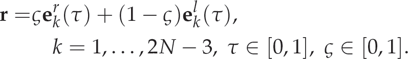
The optimal gate set G^* among all G is obtained by minimizing the performance index given by:

$$\begin{array}{ll}J(ℭ,\mathcal{G})={\displaystyle \sum _{i=1}^{n_c-2}}[\hfill & J_i(g_{i-1}(h_{i-1}),g_i(h_i),g_{i+1}(h_{i+1}))+\hfill \\ \hfill & J_{n_c-1}(g_{n_c-1}(h_{n_c-1}),g_{n_c}(h_{n_c}))],\hfill \end{array}$$

(8)

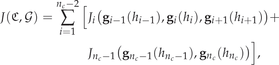
where J_i is the cost of the path segment, is represented as:

$$\begin{array}{ll}\hfill & J_i(g_{i-1}(h_{i-1}),g_i(h_i),g_{i+1}(h_{i+1}))\hfill \\ \hfill & =c_l{\overline{L}}_i-c_c{\overline{C}}_i+c_k{\overline{K}}_i,i=1,\dots ,n_c-2\hfill \\ \hfill & J_{n_c-1}(g_{n_c-1}(h_{n_c-1}),g_{n_c}(h_{n_c}))=c_l{\overline{L}}_{n_c-1}-c_c{\overline{C}}_{n_c-1}\hfill \end{array}$$

(9)

The terms determining (9) are defined as follows. L_i is the arc length of g _i (h_i)g_i+1(h_i+1). C _i is the minimum distance between g _i (h_i)g_i+1(h_i+1) and the boundary of S. K_i is the minimized maximum curvature of the curve to smooth g _i (h_i)g_i+1(h_i+1) and g_i+1(h_i+1)g_i+2(h_i+2) (detailed in the next subsection). They are normalized into non-dimensional variables ${\overline{L}}_i$ , ${\overline{C}}_i$ and ${\overline{K}}_i$ , which represent (9) such that:

$${\overline{L}}_i=\frac{L_i}{\parallel s-t\parallel },{\overline{C}}_i=\frac{2C_i}{\underset{i}{{\displaystyle \max }}{l}_i},{\overline{K}}_i=\frac{K_i}{{\kappa }_{max}}\mathrm{.}$$

(10)

That is, the arc length is scaled by ||s − t||, the distance between the initial and goal position. Proximity to the obstacles is scaled by max _i l _i /2, the maximum of half the corridor widths. The curvature is scaled by κ _max , the maximum admissible curvature of the vehicle. The normalized variables are tuned by weighing the factors c _l , c _c , c _k ∊ ℝ⁺. If any part of g _i (h_i)g_i+1(h_i+1) is outside the route in-bounds area S, then the cost of the segment is set to infinity.

The optimal gates set G^* is computed such that its corresponding path $ℛ(ℭ,{\mathcal{G}}^{*})$ has the minimum cost of (8). This paper applies DP to obtain G^*. The optimization procedure goes backwards from $g_{n_c-1}$ to g₁. Since the planned path ends at $g_{n_c}(1)$ , every gate on g _{n c-1} must point to g _{n c} (1). That is, the next gate pointer of g_{n c -1} (h_{n c -1}), denoted by d_{n c -1} (h _{n c-1} ), is given by:

$$d_{n_c-1}(h_{n_c-1})=1,\forall h_{n_c-1}=1,\dots ,M\mathrm{.}$$

The optimal cost at h_{n c -1} on g_{n c -1} to g _{n c} (1), denoted by $J_{n_c-1}^{*}[h_{n_c-1}]$ is given by:

$$J_{n_c-1}^{*}[h_{n_c-1}]=J_{n_c-1}(g_{n_c-1}(h_{n_c-1}),g_{n_c}(1))\mathrm{.}$$

Once J_{n c -1}^* for all h_{n c -1} are computed, the optimal cost at h_{n c -2} on g_{n c -2} to g _{n c} (1) is given by:

$$\begin{array}{ll}\hfill & J_{n_c-2}^{*}[h_{n_c-2}]=\underset{h_{n_c-1}∊\{1,\dots ,M\}}{{\displaystyle \min }}[J_{n_c-1}^{*}[h_{n_c-1}]+\hfill \\ \hfill & J_{n_c-2}(g_{n_c-2}(h_{n_c-2}),g_{n_c-1}(h_{n_c-1}),g_{n_c}(d_{n_c-1}(h_{n_c-1})))]\mathrm{.}\hfill \end{array}$$

(11)

The next pointer d_{n c -2}(h_{n c -2}) will be the h_{n c -1} that leads to the minimum value of [·] in (11). This procedure is repeated using (11) and decrementing the subscripts by one until one. Next, 𝒢^* is obtained by taking the pointers from 1 to n_c − 1, in order:

$$\begin{array}{l}{\mathcal{G}}^{*}=(1,d_1(1),d_2(d_1(1)),\dots ,d_{n_c-2}(d_{n_c-3}(\cdots d_1(1)\cdots )),1)\hfill \end{array}$$

Figure 8 shows the resulting optimal PPs (dotted line segments) by turning on just one of three weights c _l , c _c or c_k in the cost function (9) for an identical S. (The PPs were smoothed (solid curves) by applying the method introduced in the next subsection.) The resulting paths clearly expose the effect of each term. Figure 8(a) shows the minimum length path by setting (c_l, c_c, c_k) = (1,0,0). Figure 8(b) shows the maximum clearance path by setting (c _l , c _c , c _k ) = (0,1,0). Finally, Figure 8(c) shows the minimum curvature path by setting (c _l , c _c , c _k ) = (0,0,1).

Figure 8.

The resulting optimal paths depending on the combination of weighing factors

Finally, let us discuss the complexity of the DP algorithm. It is important to notice that the optimal cost from each gate to the goal is obtained by evaluating the cost function (9) plus the optimal costs of the gates one step closer to the goal, as in (11). For the first and last two adjacent gate stages, there are M pairs of gates. For the other adjacent gate stages, there are M² pairs of gates. Therefore, the total number of pairs is 2M + (n _c − 2)M² and the cost function is evaluated for each pair. Note that the asymptotic complexity is O(n _c M²) but that the computational cost is very low because the cost function (9) is in closed-form.

2.3. Path Smoothing

PP is discontinuous in the first derivative at each intermediate node (Figure 6), and thus does not guarantee kinematic feasibility of the robot in tracking the path. It is thus necessary to smooth PP so that it is feasible. We make a smooth connection at an intermediate node of PP by using a quadratic Bézier curve Q(λ), which is determined by three control points q₀, q₁, q₂ such that:

$$Q(\lambda )=(1-\lambda {)}^2{q}_0+2\lambda (1-\lambda )q_1+{\lambda }^2{q}_2,\lambda ∊[\mathrm{0,1}]\mathrm{.}$$

Figure 9 visualizes the method. The curve to smooth two line segments r _i , r_i+1 and r_i+1 r_i+2 is denoted by Q[i] with its control points q₀[i],q₁[i],q₂ [i]. Bézier curves have the property of being tangent to the lines between the first two and the last two control points [26]. So, we set q₁ [i] equal to the joint node r_i+1 and choose q₀[i] and q₂[i] on the line segments r _i r_i+1 and r_i+1 r_i+2. As a result, the curve is connected to the remaining path segments and is continuous in the first derivative at its end nodes.

Figure 9.

Path smoothing: Each node of a piecewise linear path is smoothed by a quadratic Bézier curve

To prevent each curve from overlapping any other, the end positions are bounded by:

$$\begin{array}{l}{\tilde{q}}_0[i]=\{\begin{array}{ll}s,\hfill & i=1,\hfill \\ \frac{r_i+r_{i+1}}{2},\hfill & i=2,\dots ,n_c-1,\hfill \end{array}\\ {\tilde{q}}_2[i]=\{\begin{array}{ll}\frac{r_{i+1}+r_{i+2}}{2},\hfill & i=1,\dots ,n_c-2,\hfill \\ t,\hfill & i=n_c-1.\hfill \end{array}\end{array}$$

From now on, let us drop the index [i] for simple notation. With the constraints set out above, Q has two degrees of freedom, represented as (α, β), the lengths between control points:

$$\begin{array}{ll}\alpha \hfill & =\parallel q_0-q_1\parallel \le \parallel {\tilde{q}}_0-q_1\parallel ,\hfill \\ \beta \hfill & =\parallel q_2-q_1\parallel \le \parallel {\tilde{q}}_2-q_1\parallel \mathrm{.}\hfill \end{array}$$

(12)

Bézier curves have another useful property of being within the convex hull of their control points [26]. This property yields that, if $\text{Δ}{\tilde{q}}_0{q}_1{\tilde{q}}_2$ lies within the constrained in-bounds area S, then Q determined by any (α, β) subject to (12) is collision-free. Otherwise, to guide Q within S, it is necessary to find an additional point $p∊\text{Δ}{\tilde{q}}_0{q}_1{\tilde{q}}_2$ such that ${\tilde{q}}_0{q}_1{\tilde{q}}_{2}p$ is the tightest tetragonal concave polygon inside S, as shown in Figure 9. In order to give smoothness to the resulting path, we should calculate (α^*, β^*), which minimizes the maximum curvature of Q with the boundary constraint. Our prior work [27] provides Algorithm 1 for finding the optimal solution:

Algorithm 1 Compute (α^*, β^*) minimizing the maximum curvature of Q with the obstacle avoidance constraint. [27]

Require: ${\tilde{q}}_0,{\tilde{q}}_0,q_{1,}$ , and $p\in \Delta {\tilde{q}}_0{\tilde{q}}_1{\tilde{q}}_2.$ . Ensure: κ _max (α^*, β^*) is the minimum of the maximum curvatures of all Q that lies within ${\tilde{q}}_0{\tilde{q}}_1{\tilde{q}}_{2}p$ . $\tilde{\alpha }\leftarrow \left|\right|{\tilde{q}}_0-q_1\left|\right|,\tilde{\beta }\leftarrow \left|\right|{\tilde{q}}_2-q_1\left|\right|$ $\theta \leftarrow \pi -\angle {\tilde{q}}_0{q}_1{\tilde{q}}_2$ $\begin{array}{l}\Xi \leftarrow \left(-\cos \theta +\sqrt{{\cos }^2\theta +8}\right)/2\\ K_a\leftarrow \frac{p_y}{\sin \theta },K_b\leftarrow p_x+p_y\cot \theta \\ {\beta }_p\left(\tilde{\alpha }\right)\leftarrow \frac{K_a}{{\left(1-\sqrt{K_b/\tilde{\alpha }}\right)}^2},{\alpha }_p\left(\tilde{\beta }\right)\leftarrow \frac{K_b}{{\left(1-\sqrt{K_a/\left(\tilde{\beta }\right)}\right)}^2}\\ {\alpha }_c\leftarrow {\left(\sqrt{K_b}+\sqrt{\frac{K_a}{\Xi }}\right)}^2\\ a_m\leftarrow {\left(\sqrt{K_b}+\sqrt{\frac{K_a}{|\cos \theta |}}\right)}^2\end{array}$ if $\Delta {\tilde{q}}_0{q}_1{\tilde{q}}_2$ is collision-free or $\tilde{\beta }\le {\beta }_p\left(\tilde{\alpha }\right)$ or $\tilde{\beta }\le {\beta }_p\left(\tilde{\alpha }\right)$ or $\Xi \tilde{\alpha }\le {\beta }_p\left(\tilde{\alpha }\right)<\tilde{\beta }$ or $\Xi \tilde{\beta }\le {\alpha }_p\left(\tilde{\beta }\right)<\tilde{\alpha }$ then $\left({\alpha }^{*},{\beta }^{*}\right)\leftarrow \left(\min (\tilde{\alpha },\Xi \tilde{\beta }),\min (\tilde{\beta },\Xi \tilde{\alpha })\right)$ else if ${\alpha }_m\le {\alpha }_p\left(\tilde{\beta }\right)<\Xi \tilde{\beta }$ then $\left({\alpha }^{*},{\beta }^{*}\right)\leftarrow \left({\alpha }_p\left(\tilde{\beta }\right),\tilde{\beta }\right)$ else $\begin{array}{l}{\alpha }^{*}\leftarrow \arg {\min }_{\alpha }\frac{{\left({(\sqrt{\alpha }-\sqrt{K_b})}^4-2K_a\cos \theta {(\sqrt{\alpha }-\sqrt{K_b})}^2+K_a^2\right)}^{\frac{3}{2}}}{2K_a^2{\sin }^2\theta {\left(\sqrt{\alpha }-{\sqrt{K}}_b\right)}^2\alpha },\hfill \\ \forall \alpha \in \left[\max \left({\alpha }_c,{\alpha }_p\left(\tilde{\beta }\right)\right),\min \left({\alpha }_m,\tilde{\alpha }\right)\right]\hfill \\ {\beta }^{*}\leftarrow {\beta }_p\left({\alpha }^{*}\right)\hfill \end{array}$ end if

The number of nodes to construct PP, n _r , has relevance to the smoothness of the resulting path. Figure 10 shows examples of the resulting smoothed paths (SP) for an identical S. In each figure in the left column, the dashed line segments and bold solid curves indicate PPs and their SPs. In Figure 10(a), PP is constructed by 5 nodes. Each intermediate node is chosen from each corner cell S_2i and is determined by cutting the edge parameters τ _i = 0.5 and ς _i = 0.5 for all i = 1,2,3. The PP of Figure 10(c) is constructed by adding each node selected from each straight cell with τ = 0.5 and ς = 0.5 to the PP in Figure 10(a). The last PP in Figure 10(e) is constructed by adding two nodes selected from each cell with (τ, ς) = (0.25,0.5) and (0.75,0.5) to the PP in Figure 10(c).

Figure 10.

Left column: The smoothed paths (bold solid curves) for primitive paths (dashed line segments). Right column: The curvature κ along the paths.

It is important to notice that as the number of nodes becomes larger, SP converges towards PP. As a result, SP tends to have a sharper corner around the nodes. This is clearly shown in the plots of the curvatures along the SPs in Figure 10(b), 10(d) and 10(f). To generate a smooth path, therefore, it is desirable to construct PP using as few nodes as possible. Intuitively, each corner of S would require a change of each curvature. So, without considering obstacles, PP is constructed by selecting one node in each corner cell, as in Figure 10(a).

2.4. Static Obstacle Avoidance

Let us extend the introduced path planning to consider static obstacles and the initial/final heading constraints. Let v₀ and v _f denote the initial and final velocities. For the sake of simplicity, we assume that the shapes of all obstacles can be bounded by a circle of appropriate radius. The path planning problem is considered in C_obstacle such that the vehicle is reduced to a point by inflating the obstacle radius to half the vehicle width.

The first step is to set gate stages. To satisfy the initial (or final) heading constraint, a finite number of gates are generated on the line segment that originates at s (or t) with a length of d_v and pointed along with v₀ (or v _f ), as shown in Figure 11(a). If the line segment intersects with the outer boundary, it is truncated by the intersection point, as shown in Figure 11(b). The gates within the same cell are grouped into a single stage.

Figure 11.

Gate stages and channels are constructed to produce a safe path over the mission route (MR) with static obstacles

Recall that a cutting edge is specified by the longitudinal position ratio τ ∊ [0, 1] between two barricades, as shown in Figure 5. So, the cutting edge that passes through the centre point of each obstacle is determined by inversely finding the τ corresponding to the point. Intuitively, the robot may require a curved trajectory to bypass each obstacle. The members of the set of gates on each cutting edge passing through an obstacle are assigned together as an individual stage. A finite number of gates are generated in each corner cell such that they do not intersect with any obstacle, as in the previous section. Figure 11(c) shows the path obtained by applying the algorithm, presented in Section 2.2, on the generated stages. Note that when an obstacle intersects with a corner cell, the gate stage of the cell is replaced by the points on the line segment through the obstacle.

In the real world, many path planning problems are for an unknown and dynamically changing environment, due to sensor limitations. Let us consider the path planning problem of a robot that has sensors capable of detecting obstacles within a limited range. We assume that the parameters W and L that specify the mission route S are initially given. In the problem, every time obstacles that intersect the pre-calculated reference path are detected, the robot must re-plan the path in order to avoid them.

Recall that two successive line segments of PP are smoothed by a quadratic Bézier curve bounded by the tetragonal polygon ${\tilde{q}}_0{q}_1{\tilde{q}}_{2}p$ (Figure 9). Similarly, every time an obstacle is added to C_obstacle, as detected, it is necessary to devise a new method to construct the tightest tetragonal polygon to avoid the obstacles. Figure 12 shows the geometry of the problem. For the obstacles that intersect the triangle ${\tilde{q}}_0{q}_1{\tilde{q}}_2$ , tangential lines are drawn from ${\tilde{q}}_0$ and ${\tilde{q}}_2$ . Thus, p is determined by the intersection of two tangential lines that have the smallest heading differential from ${\tilde{q}}_0{q}_1$ and ${\tilde{q}}_2{q}_1$ .

Figure 12.

Given $\{{\tilde{q}}_0,q_1,{\tilde{q}}_2\}$ on PP, the obstacle avoiding polygon ${\tilde{q}}_0{q}_1{\tilde{q}}_{2}p$ is determined by two tangential lines from ${\tilde{q}}_0$ and ${\tilde{q}}_2$

Figure 13 shows the snapshots of the re-planning process, consisting of a known mission and 3 unknown obstacles. The sensor detection range is illustrated by the light shaded region in the figure. An obstacle is assumed to be detected if the centre point of it lies within the sensor range cone. Given the initial information to specify the mission route in-bound area, the reference path is planned using the algorithm presented in Section 2.2 (Figure 13(a)). Since the robot sensor does not detect any obstacles, all the gate stages except for the first and the last are created in corner route cells. Thus, there is only one channel (g₁,g₂,g₃,g₄,g₅). The subscripts of the stages are assigned in order along the centre lines connecting waypoints from w₁ to w _N . At the bottom of the figure is the connectivity graph representing the adjacency relation between stages. Each vertex represents the subscript of a stage, and the stages in neighbouring cells are connected. When a new obstacle is detected as the robot moves down the reference path, the vehicle calculates whether the path intersects with the detected obstacle. If so, the path is re-planned by re-applying the algorithm. In the re-planned process, z _init is replaced with the current state of the robot and the gate sets are created for the newly detected obstacle and the current state (Figure 13(b)). The beauty of DP is that the information about the optimal paths further ahead of the obstacle can be reused for re-planning the safe path. When the robot detects an obstacle that does not intersect the path, it keeps tracking the path. This process is repeatedly performed until the vehicle reaches t (Figure 13(c)).

Figure 13.

Snapshots of static obstacle avoidance in a semi-structured environment, using DP

3. Control

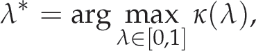
Given a reference path produced by the path planner, the trajectory generator computes the desired states as a function of time by determining a velocity profile along the path. Lepetic et al. [28] have proposed the highest allowable overall velocity profile scheme along a spline-based path with the acceleration limits of the robot, (2). We extend this method along the Bézier curve-based path with acceleration limits as follows.

The maximum curvature of a quadratic Bézier curve Q specified by α = ||q₀ − q₁||, β = ||q₂ − q₁|| and θ = π − ∠q₀q₁q₂ is determined by the Bézier parameter λ^* given by:

$${\lambda }^{*}=\{\begin{array}{ll}0,\hfill & \text{if }\frac{\alpha }{\beta }\le \cos \theta \hfill \\ 1,\hfill & \text{else if }\frac{\beta }{\alpha }\le \cos \theta \hfill \\ \frac{\alpha (\alpha -\beta \cos \theta )}{{(\alpha -\beta \cos \theta )}^2+{(\beta \sin \theta )}^2},\hfill & \text{else}\hfill \end{array}$$

such that:

$${\lambda }^{*}=\arg \underset{\lambda ∊[\mathrm{0,1}]}{{\displaystyle \max }}\kappa (\lambda ),$$

which has been derived in [27]. Q (λ^*), the point which has the maximum magnitude of curvature, is called the turning point (TP), as shown in Figure 14(a). Since TP attains a local maximum curvature, the velocity at the point should be the lowest, locally (i.e., the tangential acceleration is 0). Before and after a TP, the vehicle can move faster because the curvature is smaller than at the TP. In other words, before and after the TP, the vehicle must tangentially decelerate and accelerate, respectively [28]. Calculate the maximum allowable velocity at TP considering the limit on radial acceleration given by (2). Leaving from the point along the planned path, the velocity must vary as maximally allowed by the tangential and radial acceleration constraints with the local curvature. The maximum velocity profiles are calculated from s in a forward direction and from t in a backwards direction, along the path. The highest allowable overall velocity profile is determined as the minimum of all velocity profiles, as indicated by bold curves in Figure 14(b).

Figure 14.

The highest allowable velocity profile computation

The steering command to track the desired trajectory is generated by applying the pure pursuit-based method [29]:

$$\kappa =\frac{2\sin \eta }{L_1},$$

where L₁ is the look-ahead distance at which the reference point is on the desired path in front of the vehicle. η determines the central angle of the circular arc trajectory of the vehicle at each time step. (See Figure 15.) An important choice in the guidance law is L₁. Park et al. have provided a linear system analysis to show that L₁ must be less than about a quarter of L_p (the wavelength with the highest frequency content in the desired path) for the vehicle to accurately follow the desired path [29].

Figure 15.

Diagram for the guidance law [29]

4. Moving Obstacle Avoidance

The path planning algorithm proposed in Sections 2 and 3 maintains a balance between path optimality and computational efficiency in dealing with static obstacles. However, when the vehicle operates in a workspace filled with mobile obstacles, computational efficiency may become more crucial than motion optimality for the safety of the vehicle. This section proposes a VO-based manoeuvre for real-time moving obstacle avoidance.

4.1. Velocity Obstacle

The velocity obstacle [23], loosely stated, should match the relative velocity of the obstacle and the robot such that the robot will miss the obstacle if neither change their relative velocities. This is a set of robot's velocities that will produce a “safe escape” from the obstacle.

Let A and B denote the robot and a moving obstacle, respectively. They are considered in C_obstacle for A due to B so that A is reduced to a point, v _A and v _B denote the velocities of A and B. The relative collision cone CC _B ^A of B to A is formed by the set of the relative velocity of A, v _A − v _B , which is guaranteed to cause a collision between A and B [23]. Assuming a constant velocity, the velocity obstacle VO _B ^A is obtained by translating CC _B ^A of the vector v _B . So, any velocity of A, v _A that remains within VO _B ^A will result in a collision, at some moment in time, with B. VO _B ^A is represented as follows [25]:

$$V{O}_B^A=\left\{v_A\right|\rho (A,v_A-v_B)\cap B\ne \varnothing \},$$

where ρ(p,v) denotes the ray originating at p and in line with v.

$$\rho (p,v)=\{p+tv|t\ge 0\}$$

Figure 16(a) shows the geometry of the Velocity Obstacle. When v _A lies inside of VO _B ^A , t _c , the time to collision can be calculated by equating ρ(A, v _A − v _B ) and ∂B, the boundary of B [25]:

Figure 16.

The paradigm of Velocity Obstacle

$$t_c(v_A)=\min t,\forall t∊\left\{t\right|A+t(v_A-v_B)=\partial B\}\mathrm{.}$$

To estimate the safety of the robot against obstacles, we define some notation in the Velocity Obstacles paradigm. When v _A lies outside of VO _B ^A , the time to possible collision t _pc is defined as the minimum possible time for A to collide with B by changing heading while keeping the magnitude of v _A constant:

$$t_{pc}(v_A)=\frac{\parallel A-B{\parallel }_{min}}{\parallel v_A-v_B\parallel },$$

where ||A − B|| _min is defined as the minimum distance between A and any point of B. For example, ||A − B|| _min for the circular obstacle B, with the radius of r given by:

$$\parallel A-B{\parallel }_{min}=\parallel A-B\parallel -r\mathrm{.}$$

Also, ϑ(v _A ) is defined as the minimum angle difference of v _A − v _B and CC _A ^B , as shown in Figure 16(b).

4.2. Obstacle Avoidance Manoeuvre

Let v _A [k] denote the discretized velocity of A at t = kΔt, where Δt is the time step:

$$v_A[k]:=v_A(k\text{Δ}t)\mathrm{.}$$

The moving obstacle avoiding manoeuvre can be treated as selecting vA[k],k = 1,2,… such that A safely navigates towards its goal when the trajectory is generated by the selected set of velocities with the given initial position and velocity.

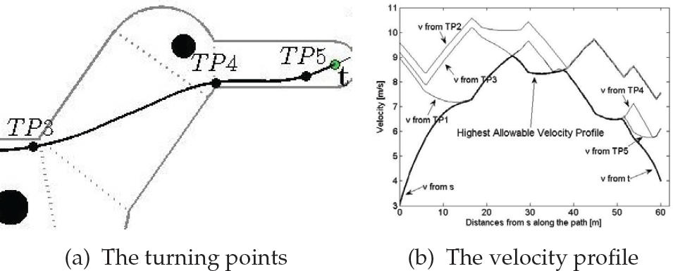
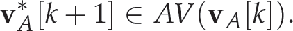
Given the current velocity v _A [k], the kinematic and dynamic constraints imposed on the robot A restrict the set of admissible velocities at next sample time, v _A [k + 1]. The set denoted by AV (v _A [k]) is represented as:

$$\begin{array}{l}AV(v_A[k])=\left\{v\right|\\ v_{min}[k]\le \parallel v\parallel \le v_{max}[k]\wedge \frac{|\angle v-\angle v_A[k]|}{\text{Δ}t}\le {\omega }_{max}[k]\},\end{array}$$

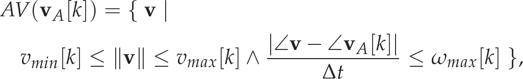
where the maximum and the minimum magnitude of velocity, v_max and v_min, and the maximum yaw rate ω _max at t = kΔt, are determined by the limits on tangential and radial acceleration, a _tMax and a_rMax, of the robot:

$$\begin{array}{l}{v}_{max}[k]=\parallel v_A[k]\parallel +a_{tMax}\text{Δ}t\\ v_{min}[k]=\parallel v_A[k]\parallel -a_{tMax}\text{Δ}t\\ {\omega }_{max}[k]=\frac{a_{rMax}}{\parallel v_A[k]\parallel }\mathrm{.}\end{array}$$

Figure 17 shows the geometry of AV(v _A [k]), as illustrated in the shaded sector. Then, v _A [k + 1] must be selected from AV(v _A [k]):

Figure 17.

Geometry of the admissible velocities

$$v_A[k+1]∊AV(v_A[k])\mathrm{.}$$

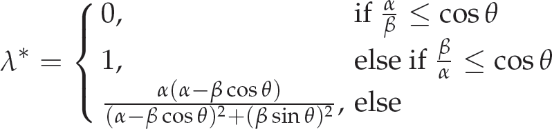
For the purpose of the computation of the optimal feasible velocity at each time step, AV(v _A [k]) is sampled into n _t n _r points, called the candidate velocities, as indicated by the dots in Figure 17, where n_t and n_r are the number of sample points in the tangential and radial directions with respect to v _A [k]. The candidate velocity v _A [k+1](i, j), i = 1,…, n_t, j = 1,…, n _r is given by:

$$\begin{array}{l}\parallel v_A[k+1](i,j)\parallel =\frac{i-1}{n_t-1}(v_{max}-v_{min}),\\ \angle v_A[k+1](i,j)=\angle v_A[k]+(\frac{2(j-1)}{n_r-1}-1){\omega }_{max}\text{Δ}t\mathrm{.}\end{array}$$

The cost of a candidate velocity v _A [k + 1](i,j) against an obstacle B is given by:

$$\begin{array}{l}{J}_o(v_A,B)=\{\begin{array}{ll}{c}_{in}\frac{1}{t_c(v_A)},\hfill & \text{if}{v}_A∊V{O}_B^A,\hfill \\ -c_{out}\frac{\vartheta (v_A)}{t_{pc}(v_A)},\hfill & \text{otherwise,}\hfill \end{array}\hfill \end{array}$$

(13)

where [k + 1] (i,j), the index of v _A , is dropped for notational simplicity. Note that when v _A is within VO _B ^A , the cost rewards t_c for v _A to escape from the area VO _B ^A . Otherwise, it penalizes ϑ in an inverse proportion to t_pc. This is because penalties on ϑ guide v _A to head farther away from VO _B ^A , and the penalties are more critical for smaller t _pc . The two terms are tuned by weighing factors c_in and c_out.

The route boundaries ∂S can be considered as static obstacles, i.e., ones that have no velocity. For example, as illustrated in Figure 18, when A is within a straight route cell bounded by c _l ,c _r , d _l ,d _r , the left and right boundary line segments, c _l d _l and c _r d _r , can be considered as obstacles, as denoted by o _l and o _r . Since the velocity of o _l is zero, the velocity obstacle VO _{o l} ^A originates at A and is bounded by Ac _l and Ad _l , and so forth, for o _r . The cost of the velocity v _A against the obstacles is obtained by replacing B with o _l or o _r in (13).

Figure 18.

Velocity obstacles against the in-bounds area

To make the robot A move towards the target point t under the corridor constraint, an additional cost is introduced. Let L denote the leaving barricade of the route cell in which A is located. VO _L ^A can be constructed as though L were a static obstacle, as shown in Figure 18. The cost of v _A to L is defined as the same (but the opposite) sign to (13):

$$J_b(v_A,L)=\{\begin{array}{ll}-c_{in}^{\text{'}}\frac{1}{t_c(v_A)},\hfill & \text{ if }{v}_A∊V{O}_L^A\hfill \\ c_{out}^{\text{'}}\frac{\vartheta (v_A)}{t_{pc}(v_A)},\hfill & \text{ otherwise}\hfill \end{array},$$

So, while J_o makes A reflective in relation to an obstacle, J_b makes it attractive in relation to the leaving barricade. For notational convenience, L is t when A is within the last route cell.

Finally, given the current velocity v _A [k] of A that is within the route cell of which the leaving barricade is L, the optimal velocity at the next time step, v _A ^* [k + 1], against the set of obstacles O = o₁,…, o _M , is obtained by minimizing:

$$J(v_A,O,L)=J_b(v_A,L)+{\displaystyle \sum _{i=1}^M}{J}_o(v_A,o_i)$$

(14)

subject to:

$$v_A^{*}[k+1]∊AV(v_A[k])\mathrm{.}$$

To incorporate moving obstacle avoidance with global path planning along the mission route (MR), we use the following approaches: as long as a moving obstacle is detected within the robot sensor range, the moving obstacle avoidance algorithm presented in this section is used by discarding the pre-calculated global path information. Once all the obstacles are out of sensor range, the reference path is re-planned by using the global path information in a receding horizon fashion.

5. Numerical Experiments

The simulations provided in this section are implemented in MATLAB and tested on a Windows PC with a Pentium IV 1800 MHz processor.

The first simulation demonstrates the proposed motion planning algorithm for the avoidance of moving obstacles (Section 4). Figure 19 shows snapshots of the real-time motion planning of the vehicle operating in a corridor determined by two vertical line objects, filled with moving obstacles. Each obstacle is illustrated as a black circle, with its corresponding velocity obstacle illustrated as a bright shaded cone. The obstacles have different sizes and their motions are modelled either linearly or circularly. The smaller and larger circles around the vehicle indicate the minimum and maximum magnitudes of the admissible velocity range respectively. The cone that originates at the vehicle indicates the admissible heading range. So, the admissible velocity is determined by the circular arc sector enclosed by the circles and the cone. The arrow that originates at the vehicle indicates the commanded velocity of the vehicle such that the tip of the arrow is within the admissible velocity area. (A video of this simulation can be found at http://www.youtube.com/watch?v=zvScrJE3k88.)

Figure 19.

Motion planning of the vehicle traversing a corridor (the two vertical line segments) for the avoidance of moving obstacles (black circles). For each obstacle, the velocity obstacle is illustrated as a bright shaded cone.

The second simulation was to demonstrate the safe motion planned by incorporating all the proposed algorithms. Figure 20 shows the mission environment, MR, filled with unknown (moving and static) obstacles on the top row. The initial path (dashed curve) is planned for the given MR by applying the proposed path planning algorithm (Section 2.2). The optimal path is obtained by equally penalizing the arc length, the proximity to obstacles and the curvature by setting (c _l , c _c ,c _k ) = (1,1,1) in the cost function (9). The rest of the images comprise snapshots of the proposed algorithms. We assume that the sensor detection range is defined as a circular sector (with a centre angle of 120° and a radius of 40m), such that the heading of the vehicle is at the bisector of its central angle. It is illustrated as the light, shaded region in the figures. An obstacle is assumed to be detected if its centre point lies inside the sensor detection range. In the initial position s, the vehicle sensor detects no obstacle in the environment. To simulate localization errors, the noise was modelled as white noise with a magnitude of 0.2m and was added to the actual position. Next, the vehicle follows the disturbed reference path by using the trajectory generation and tracking algorithm (Section 3). When new obstacles are detected as the vehicle tracks the path, the vehicle calculates whether the path intersects the obstacles. If so, it is necessary to manoeuvre depending on whether one of the detected obstacles is moving. When the vehicle runs into moving obstacles, the motion is planned by using the method presented in Section 4 After the vehicle's velocity escapes from the area, the reference path is re-planned by applying the path planning algorithm in a receding horizon fashion (Section 2.4). This process is repeatedly done until the vehicle reaches t. (Video of the result can be found at http://www.youtube.com/watch?v=pqu9M_XXeD0.)

Figure 20.

Snapshots of real-time obstacle avoidance motion planning of the robot operating in a semi-structured environment

Figure 21(a) and 21(b) show the control command history. The plots of the tangential and radial acceleration correspond to the control, while Figure 21(c) and 21(d) show that the vehicle satisfies its tangential and radial acceleration constraints: a_tMax = 3m/s² and a_rMax = 5m/s². Our methods are all robust to this kind of motion due to the fast path re-planning.

Figure 21.

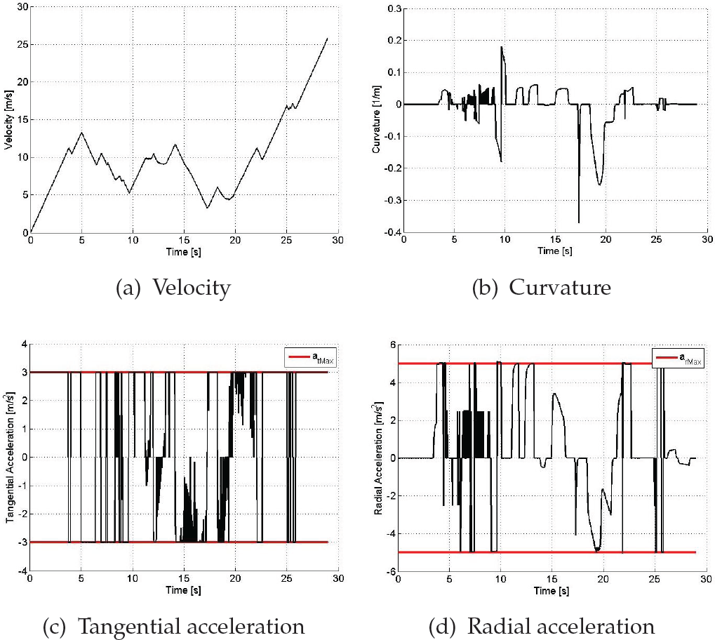
Control command history and tangential and radial acceleration exerted by the control command

6. Summary

This paper proposes a real-time motion planning algorithm for autonomous ground vehicles operating in semi-structured environments. The algorithm switches between two kinds of planners depending on the mobilities of detected obstacles.

The first planner, for static obstacle avoidance, combines a path planner and a controller. The first step of path planning is to decompose the mission route specified by waypoints and corridor widths into discrete cells. We introduce the cutting edges method to efficiently re-decompose C_free in a dynamically changing environment. Each cutting edge is determined by dividing ratio values on the boundary of C_free. The decomposed route cell and the cutting edges passing through obstacles are discretized into a finite number of points. The optimal piecewise linear path is then determined by connecting a subset of the points with the use of dynamic programming (DP). DP reduces the re-planning computation time by enabling the path planner to reuse pre-calculated global shortest path information. The next step is to smooth the path based on Bézier curves such that the maximum curvature of each curve is minimized with a polygonal boundary constraint. The efficiency and performance of the proposed path smoothing method is demonstrated.

The controller calculates the maximum allowable velocity profile from turning points (TP) along the path, satisfying limits on the maximum tangential and radial acceleration of the vehicle and based on the path provided by the path planner. The analysis of the maximum curvature of a quadratic Bézier curve assists the efficient calculation of the TP. The highest allowable velocity profile is determined as the minimum of all velocity profiles. Next, control commands are generated for the vehicle to accurately track the desired trajectory by using a pure pursuit-based nonlinear trajectory tracking guidance law.

To efficiently operate in an environment filled with moving obstacles, the second planner produces time-optimal motions by incorporating dynamic constraints during motion planning. More specifically, to satisfy the waypoints and corridor constraints, we compute the sequence of velocities, in discrete time, which minimizes the cost determined by expected collision times, the safety of the current velocity against obstacles, and the deviation of the current velocity relative to the desired velocity. The algorithm is incorporated with global path planning. Our numerical simulations demonstrate that these algorithms generate successful motions for autonomous vehicles with a limited sensor range while meeting the maximum allowable tangential and radial acceleration constraints.