
Abstract
The Szabad(ka)-II 18 DOF walking robot and its simulation model is suitable for research into hexapod walking algorithm and motion control. The complete dynamic model has already been built, and is used as a black box for walking optimization in this research. First, optimal straight line walking was chosen as our objective, since the robot mainly moves in this mode. This case can be tested and validated as well on the current version of our robot. An ellipse-based leg trajectory has been generated for this low-cost straight line walking. Currently a simple new Fuzzy-PI controller with three input variables is being constructed and compared with an previously used PI controller. The purpose of defining the rules and its optimization are to obtain a controller that provides walking with higher quality. Both the compared controllers have been optimized together with the parameters of the leg trajectory. The particle swarm optimization (PSO) method was chosen from several methods with our benchmark-based selection research and the help of specific test functions; moreover the previous research (the comparison of genetic algorithm (GA) and PSO) also led to this conclusion.
Introduction
This research contributes to the development of the driving control optimization of the Szabad(ka)-II mechatronic device [1–7]. It deals with two issues: 1) finding a relatively quick optimization method for a non-differentiable and highly non-linear objective, i.e., the simulation model of the Szabad(ka)-II robot; 2) optimizing hexapod walking with the help of the simulation model in order to achieve an adequate trajectory curve and an effective Fuzzy motor control that can be later embedded into the robot's microcontrollers. However finding a certain optimal solution was not the focus; rather, the goal was to obtain a new procedure that can be generally applied for the tuning of robot controllers if the simulation model is available.
The improvement of the robot's walking on rough terrain is still in progress, including the designing of new legs containing ground contact sensors. In the current research phase a relatively simple case - the straight-line tripod walking on flat ground - was selected first to develop the optimization system of the robot motion and control. In order to obtain optimal parameter values, which can be used for the building or design of a real robot, a proper robot model is required.
The current simulation model was introduced in [3], which is a detailed kinematic and dynamic model of the real Szabad(ka)-II robot (Fig. 1). The aim of this model is to simulate the motion, and measure the walking quality (also known as performance) in comprehensive situations. Controller optimization with the help of the model is important because the system's performance mostly depends on the controller's efficiency [9] besides the structural parameters. Numerous research studies have defined the necessity and role of simulation, controller optimization and fitness function, for example in the conclusion of articles [8, 38]. The controllers and walking trajectories - both developed in this model - can be implemented into the microcontroller of the real robot. The model is validated by the dynamic measurements taken on the real robot (as mentioned in [40], and to be published in detail). Thus the expected deviation between the simulation and reality is known.

Szabad(ka)-II hexapod robot
The previous research [1] constitutes the basis of this work, which compares two optimization methods (GA and PSO) on a robot-walking task with a PI controller. Some of the most successful applications of fuzzy control have been highly related to conventional controllers, such as proportional-integral-derivative (PID) controller [10]. Currently a Fuzzy-PI controller is being introduced and both the compared controllers are being tuned up with the selected optimization method. The literature provides several examples of the applicability of the fuzzy controller, and most of these also apply the optimization for tuning up Fuzzy parameters, for example: [8, 11–17]. Moreover one publication deals with PID controller optimization [9]. The main difference between fuzzy logic control (FTC) and conventional control is that the former is not based on a properly defined model of the system, but instead implements the same control ‘rules’ that a skilled expert would operate [10].
The Fuzzy inference system also proved to be suitable for the tuning of the sliding mode control [18], especially in the case of a non-linear system. Hexapod robots also have a strongly non-linear and variable dynamic character, thus the effective control with a Fuzzy type system is expected.
Fitness function
The most suitable optimum can be obtained primarily if the quality definition is correctly determined. The specific robot's walking optimality is measured by a certain fitness function (also known as cost- or objective function). In the previous research a fitness function was already defined and used for the same problem [1, 5].
The tripod type [19] straight-line hexapod walking on even ground is a simpler case. It has been assumed that in such a case the robot moves towards a farther target point without any manoeuvres and other operations. More energy would remain for the other walking modes if the energy consumption was minimized for straight line walking. Thus the most important task will be to achieve a fast and low-cost (low energy consumption) locomotion. The presented fitness function (1) expresses the quality measurement of these features. It is a concrete aggregation of multi-objectives resulting in a global criterion (F) based on the weighted product method. Generally the goals of robot walking are [5]:
achieving the maximum speed of walking with as little electric energy as possible, similarly to [20],
keeping the minimal torques on the joints and gears,
maintaining the currents of the motors as little discursive and spiky as possible, and
keeping the robot's body acceleration at a minimum in all three-dimensional directions.
In order to obtain the results in accordance with our demands, the following should be emphasized (1): In the fitness function the average velocity tag was squared in order to emphasize it as much as the small energy consumption and the accelerations, i. e., these two aspects influence the system oppositely.

where
The tripod-type hexapod walking [19] is the most appropriate for a fast and low-cost locomotion. For this walking a three-dimensional ellipse-based trajectory curve was generated that defines the feet's desired cyclic movement in relation to the robot body. More detailed description of this deformed half-ellipse trajectory can be found in [4].
The trajectory curve and the driving motor controller's behaviour directly influence both the real or simulated movement. Since the change of the trajectory's parameters will influence the optimal values of the other parameters – that is, the parameters are not independent – the optimal parameter set should be found in the multi-dimensional space. Therefore the chosen motor controllers and the parameters of this trajectory (see Table 1) have been optimized together. The similar trajectory optimization attempt in [20] did not optimize the motor controller with this trajectory; this is what is different in the current research. The lower (min.) and upper (max.) bounds of these parameters were defined empirically in most cases, with the exception of the upper bound of the fourth ‘length of the step’ (T B ) parameter given by the structural dimension of the robot.
Trajectory parameters and its bounds
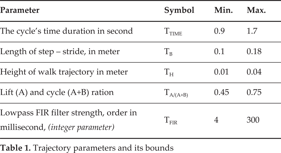
Trajectory parameters and its bounds
This paper further describes an effort to search for the best optimization method that can most effectively solve the mentioned problem (the best result in terms of performed time and achieved fitness value).
The optimization speed is very important for our system, because the simulation of one second with Szabad(ka)-II dynamic model takes four minutes in an up-to-date PC with a i7-2600K processor (i.e., Simulink solver with 0.2ms time step, model of 18 DC motor, 18 inverse dynamics, etc.). This means one optimization process lasts for several days, and searching for the best optimization method with adequate parameters would last several months.
Chapter 2 briefly presents the benchmarking of the optimization methods applied on different test functions. Multi-dimensional quick test functions have been selected for the benchmark, which have similar non-linear, discontinuous, integer, etc. characters as in the case of the walking simulation of the Szabad(ka)-II robot. Based on the research in Chapter 2 the best possible optimization method could be chosen for the current robot walking.
Selection of optimization methods
There are numerous multi-parameter optimization methods, and it is generally difficult to choose the best because the performance of each method is problem-dependent [21]. Based on our experience [1, 4, 5] and literature [8, 21–24] the heuristic and hybrid methods are promising for a non-linear, multi-parameter system. Table 2 lists the selected methods that are currently under test and comparison. Moreover while trying to select the best method the existence of public Matlab implementation [25–30] was taken into account in order to avoid algorithm implementation and obtain quick results:
Selected optimization methods for the benchmark on test functions
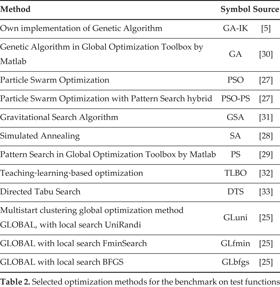
Selected optimization methods for the benchmark on test functions
Genetic algorithm (GA) can be applied to solve problems that are not well suited for standard optimization algorithms, including problems in which the objective function is discontinuous, non-differentiable, stochastic, or highly nonlinear [30].
Particle swarm optimization (PSO) is one of the most important swarm intelligence paradigms [12]. The PSO uses a simple mechanism that mimics swarm behaviour in bird flocking and fish schooling to guide the particles to search for globally optimal solutions [16]. There is no built-in PSO algorithm in Matlab, and thus external source exploration was needed. Considering the characteristics of the available implementations, [27] seems to be the good choice. It is easy to learn, has the ordinary Matlab-like syntax, and has only the necessary options.
The pattern search (PS) algorithm supported in Global Optimization Toolbox by Matlab [29].
Gravitational search algorithm (GSA) is a never-heuristic optimization method, which is constructed based on the law of gravity and the notion of mass interactions [31].
Simulated annealing (SA) models the physical process of heating a material and then slowly lowering the temperature to decrease defects, thus minimizing the system energy [28].
Teaching-learning-based optimization (TLBO) is a population-based, new, efficient optimization method, which works on the effect of the influence of a teacher on learners. [32]
Tabu search (TS) is a heuristic method but is still very limited for dealing with continuous problems. The directed tabu search (DTS) is a continuous TS that also uses the Nelder-Mead method and adaptive pattern search. [33]
The new version of ‘multistart clustering global optimization method’ (called GLOBAL) utilizes the advantages offered by Matlab, and the algorithmic improvements increase the size of the problems that can be solved reliably with it [25].
Not all the selected optimization methods with various configurations are worth running on the simulation model of the Szabad(ka)-II robot, because it would take half a year (see chapter 1.4). This led to the application of the methods’ benchmark on faster test functions, and offered a kind of pre-selection of methods based on some key characteristic behaviours. The current dynamic model of hexapod walking - in view of character - is a multi-dimensional, highly nonlinear, non-smooth, and a slightly mixed integer problem, i.e., it:
Has a minimum of seven dimensions: PI controller has seven dimensions (5 trajectory+2 PI parameters), while the Fuzzy-PI has 17 dimensions (5 trajectories+12 Fuzzy parameters).
Has non-continuous behaviour due to walking on six legs and the ground contact.
Has no random parts.
Contains integer parameters, e.g., the trajectory parameter T FIR is an integer type, see Table 1 and Table 4.
The ground contact model of the six legs - a critical part of the dynamic model - has a discontinuous character as it can be seen in formulae (2), (3) and (4). More details about this ground contact model can be found in [3, 7]. The backlash occurrence at the robot's links and gears also has a non-smooth feature.


Therefore test functions have been selected based on the mentioned aspects in order to ensure the testing of these characters:
smaller (marked with D4) and larger (D7) dimensions,
continuous (C1) and discontinuous (C0),
with integer (I1) and without integer (I0),
with random (R1) and without random (R0).
Both of them can be seen in formulae (5) and (6); the rest assemble from the mixing of presented function tags, the exact optimum is known, and the various methods (run with the same conditions) make efforts to find this set as much as possible. Selected methods run as constrained optimization, and the test function has been scaled in order to support unified side constraints -1 ≤ x ≤ 1, except the integer parameter, which has 0 ≤ x ≤ 10 ranges. These test functions can be downloaded from the webpage [34].
The discontinuous (C0) and seven dimension (D7) functions are more interesting for the present problem. Bearing in mind the previous facts and assumptions the D7C0R0I1 function is the closest to this simulation system as the objective function. It is expected that the robot-walking problem will be effectively optimized with the methods providing better results for such a test function that has the same characteristics as the problem. This assumption was confirmed in this example.
Each optimization method was run N=100 times with various configurations on all test functions. The configuration refers to some main parameters of a certain optimization method, which was randomly selected in each case (for example, in the case of GA: generations, population, elite count, crossover type).
Fig. 2 shows the results in case of four-dimension test functions, while Fig. 3 and Fig. 4 illustrate the seven dimension cases. The left-bottom corners represent the best performance, i.e., the better fitness on the horizontal axis and the smaller number of function calls on the vertical axis. An acceptance condition was defined, and plotted with a magenta line. Different performance clouds can be seen in cases of various types of functions. There are more methods reaching acceptable results for the four-dimension problem (Fig. 2). However, in case of seven dimensions (D7) and discontinuous (C0) benchmark only the PSO, the PSO-PS hybrid, and TLBO methods reach really acceptable results (Fig. 3 and Fig. 4). The following findings can be obtained from the clouds in Fig. 3 and Fig. 4:
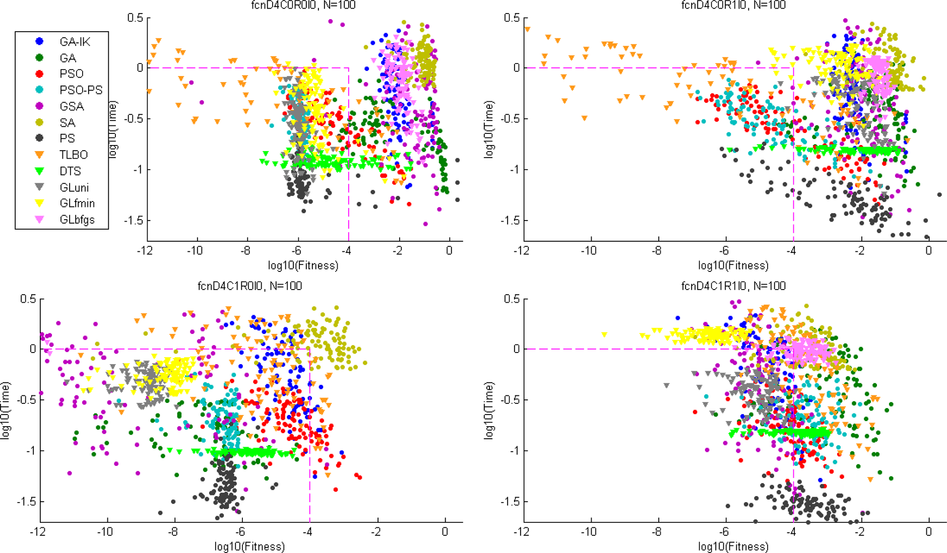
Optimization benchmark on functions of four dimensions (D4 without integer (I0)
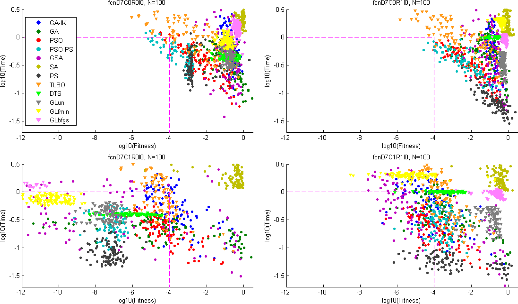
Optimization benchmark on functions of seven dimensions (D7) and without integer (I0)
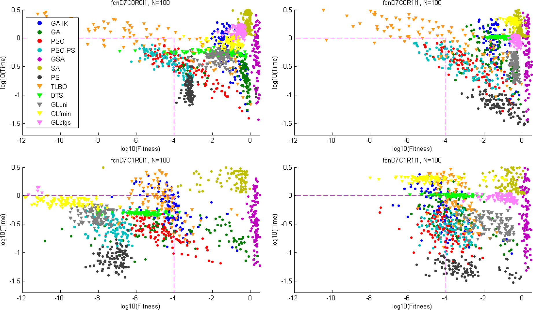
Optimization benchmark on functions of seven dimensions (D7) and with integer (I1)
The PSO, PSO-PS, and TLBO methods provide the best stable results for all the discontinuous functions.
The PSO-PS hybrid method contains the good performance of PSO and the stableness of PS. Thus this will be the best choice for higher dimension problems, especially in the case of D7C0R0I1 function (left-top graph in Fig. 4), which is most similar to the current robot model.
The GL*, PS and DTS methods reach almost the best results for the continuous functions without random tags, but in other cases give a lower performance.
The GA, GA-IK, GSA and SA methods do not reach acceptable results in any case. The SA method seems to to be the weakest for all types of functions.
The GA methods reach a lower performance but keep roughly similar values for different test functions. This reinforces the problem-independent character of GA.
The GSA method is excellent only for the continuous problems without an integer tag, but very weak for the others.


The results of this benchmark contributed and confirmed the effectiveness of the selected PSO method as mentioned in papers [1, 11, 24, 15]. Similar benchmark efforts can be found in [22] where the PSO also reaches a very good performance level. In paper [11] a benchmark of optimization methods (ANFIS, PSO among others) was also applied on a Fuzzy controller, not on the test functions. It also confirmed the PSO usability for tuning the Fuzzy system. The pattern search (PS) can refine the result from PSO (compare PSO and PSO-PS clouds in Fig. 2, Fig. 3, Fig. 4). It runs after PSO and is initialized by the best entities of PSO. Thus, the PSO-PS pair has become the best method for us.
First of all the design of a controller is primarily defined by the fact that it should be implemented into the microcontrollers of the real Szabad(ka) robot series. This means that the memory and calculation demand of the controller should be maintained within certain boundaries. From another aspect only just the available measured quantities can be used as input (of a Fuzzy controller) due to the given sensor interface.
Based on previous research [6, 35] a Fuzzy controller with some rules is enough for obtaining an improved result compared with the simple PID controller. One of the key things is the fact that Fuzzy can include more inputs, while the PID has only one (the error of control variable). In case of robot link control it is the angle error, i.e., the difference between the desired and measured angle. Besides this the absolute value of the motor current was put into the Fuzzy inputs; it was possible since the electronics on the Szabad(ka)-II measures this. A similar solution [10] was found in the literature; however the authors do not explain the role of this current feedback. In addition, if required, the derivative of angle error and the error of angle velocity could be used as input or the measured angle value might also be applied in case the controlling behaviour is different in a certain angle section.
Fuzzy inputs and outputs
The block diagram in Fig. 5 shows the designed Fuzzy-PI controlling cycle with the inputs and outputs. The three selected inputs are: error angle (A ERR ), error velocity (VERR), and motor current (IMA), while the two outputs are: proportional tag of voltage (FZZP), and integrative tag of voltage (FZZI).A controller system with the same parameters and conditions should be provided for each 18 DC motor of the robot. Currently this controller has been implemented only on the dynamic model of Szabad(ka)-II robot, when it was tested and optimized.
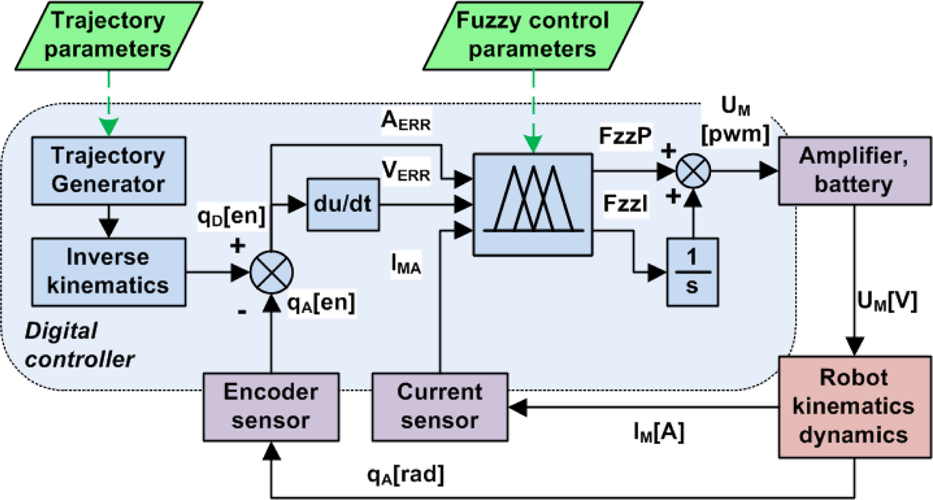
Fuzzy-PI motor control loop in the dynamic model of Szabad(ka)-II robot
Fig. 6 presents the necessary membership functions (MFs) and the eight rules defined by the authors, which mostly determine the rule rolling character:

Rules of Fuzzy-PI controller: first input column is the error angle, second input column is the absolute motor current, third column is the error, first output column is the proportional tag, and second output column is the integrative tag.
The first rule refers to cases when there is no error angle and the outputs come near to zero.
The second rule ensures that if the velocity error is small then the integration output tends toward zero.
The third and fourth rules ensures the output activity in order to decrease the control (angle) error.
The fifth and sixth rules have an opposite influence to the third and fourth rules, but only when the motor current is high. These rules ensure a softer feature of controlling when the currents or torques are great, and thus can protect against electrical and mechanical overload.
The seventh and eighth rules reinforce the integrative output activity for decreasing the velocity error when the motor current is smaller.
The logic of these rules has been reinforced by earlier research [6], but on the other hand the optimization process should select the necessary or dominant rules by tuning up its weights.
Fig. 7 illustrates the output surfaces of the built Fuzzy-PI controller, where the aggregated effects of the previously described rules can be observed.

Outputs’ surfaces of Fuzzy-PI controller, above the proportional output, below the integrative output
The number of Fuzzy controller parameters depends on the number of all MFs and rules. If it is assumed that the defined rules are suitable, then only the weight of them count as target parameters. Furthermore there is no need to count separate parameter values for the symmetric MFs and rules. According to this the current Fuzzy-PI controller has 37 parameters in all:
5 method type parameters: AndMethod, OrMethod, ImpMethod, AggMethod, DefuzzMethod
9 MFs × 3 parameters (2 scale values+1 function type value (trimf or gaussmf))
weight of 5 rules (8 rules – 3 symmetry)
Despite this the parameters of MFs have been reduced by the following method: only the range values of inputs and outputs have been changed, thus the internal MFs do not change relative to each other. For the modification of the range values it is also necessary to convert the parameters of the Fuzzy membership functions, for which the Fuzzy Toolbox's
Table 3 contains the selected 12 main parameters of the current Fuzzy-PI controller with the target domains (Min, Max columns).
Fuzzy-PI controller parameters and its target boundaries

Fuzzy-PI controller parameters and its target boundaries
The MF types of inputs have not been selected for optimization, partly because they only slightly influence the output surface, and partly because the selected shapes were intended. For example, the triangle shapes at positive MF and negative MF of angle error (AERR) are important for precise control.
Simulation
The simulation model was introduced in [3], which is a detailed and 3D kinematic and dynamic model of the real Szabad(ka)-II hexapod robot, implemented in Simulink environment with the help of Robotics toolbox [39]. It includes the exact copy of the digital controller with the trajectory generator, DC motors and gears, rigid body dynamics, the ground contacts as an approximated model, ground surface, and in some degree the sensors (encoder, current measurement, and accelerometer).
In the initial state of the chosen simulation case, the robot's bottom point was 1mm above the ground; the legs were set to the initial points of the desired trajectories. The simulation time was selected for only three seconds in order to hasten the runtime as much as possible, but at least to enable the simulation of one and a half walking cycles. The ground was even with a 0.9 friction constant. After the simulation the fitness function runs and calculates the specified quality of walking based on the simulation results (robot movements, motor currents, link torques).
Optimization results
The results of optimization can be seen in Table 4 for both controller types (PI and Fuzzy-PI), and for two optimization cases with PSO-PS and PSO methods. The PSO-PS method was selected for the current optimization case, the reason described in Chapter 2. The PSO-specific parameters were: the number of generation was selected to NG=70, the population size was NP=40, the inertia weight w=0.9, the cognitive attraction c1=0.5, and the social attraction c2=1.5. These parameters were selected partly from the literature [1, 11, 23, 21, 24, 15], partly from own experience.
Table 5 comprises the detailed partial results of the fitness evaluation (1). However, the Fuzzy-PI-PSO method seems to be the best one if only the lowest energy consumption and the fastest movement is considered. But the lower accelerations and stability are also important for the quality, and that is why our fitness function (1) takes into account all of these properties. In this respect the Fuzzy-PI-PSO-PS has the best fitness value (without any significant differences).
Optimized walking parameters: trajectory and controllers

Optimized walking parameters: trajectory and controllers
Table 5 comprises the detailed partial results of the fitness evaluation (1). However, the Fuzzy-PI-PSO method seems to be the best one if only the lowest energy consumption and the fastest movement is considered. But the lower accelerations and stability are also important for the quality, and that is why our fitness function (1) takes into account all of these properties. In this respect the Fuzzy-PI-PSO-PS has the best fitness value (without any significant differences).
Fitness values and function tags in cases of optimized PI and Fuzzy-PI system. More details can be found in [1]
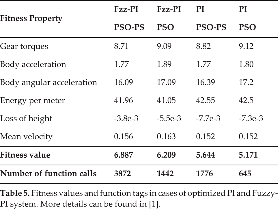
Fig. 8 shows the time diagram of the robot movement (B X ), velocity (BV X ) acceleration (BA Mag ), and the summarized motor currents (I SUM ) for five optimized cases:

Comparison of optimized walking with PI and Fuzzy-PI controllers: movement (B x ) at top-left, velocity (B vx ) at bottom-left, summarized motor current (ISUM) at top-right, and magnitude of 3D body acceleration (BA Mag ) at bottom-right
Fuzzy-PI controller optimized with PSO-PS method (red)-the best Fuzzy solution, high fitness obtained by smaller energy consumption and smaller acceleration, see Table 5.
Fuzzy-PI controller optimized with PSO method (yellow)-the Fuzzy reached a little faster movement than the PI besides a roughly same power consumption and body acceleration. This was the main reason for the higher fitness value.
PI controller optimized with PSO-PS method (blue) - the best PI solution, the details can be seen in Table 5.
PI controller optimized with PSO method (green) - an interesting trajectory can be observed, very similar to the best Fuzzy-PI solution
PI controller optimized with GA previously [1, 5] (grey) - it is important to present the mentioned typical hexapod gait problem, i.e., the significant fluctuation of velocity.
Based on the comparison of these four optimized cases and the other results obtained during the development it can be concluded that some solutions reach the high fitness value by higher speed, while others reach this value by smaller energy and acceleration. In spite of the difference between the presented four cases, both control methods in all given solutions generate high quality walking: the fluctuation of velocity is relatively small compared to a typical inadequate hexapod walking, illustrated with grey in Fig. 8, and found in [1, 5, 6]. Mostly the motor currents have different curves due to the fact that the Fuzzy also includes the current in the control decision.
The three-dimensional leg trajectory can be seen in Fig. 9, related to the five mentioned optimized cases in Fig. 8. The ellipse-based desired trajectory was also plotted with a little shift besides the simulated-regulated trajectory. The simulated-regulated angle curves of three robot leg links illustrated on the right follow the desired angle curves calculated with inverse kinematics. The explanation of the presented link numeration can be found in Fig. 3 in paper [36].

Leg trajectory curves of four optimized cases: the desired and simulated trajectory curves (left), simulated angles of three links (right)
During this research the authors gained experience in the field of robot control optimization. A new and more widely usable method was created for (pre)selecting the potentially best optimization method(s) used for a given problem. The test functions for a benchmark were created including those mathematical characteristics that are interesting or typically describe the examined objective function (chapter 2.1). The selection of these characteristics was the key point, since certain methods provide significantly different performance levels for different test functions with various characteristics (see chapter 2.2). It can be observed that the parameters of the optimization method also have an influence, because the random change of these parameters formed a cloud for each method (see coloured clouds in Fig. 2, Fig. 3, Fig. 4). The best set of these parameters can also probably be deducted from these benchmark results.
In the current demonstrated case the objective function is the straight-line walking quality of the Szabad(ka)-II robot with a Fuzzy controller in virtual simulation space using the dynamic model. The design vector (parameters to be optimized) of this system contains both parameters of the trajectory and the controller. If the optimization methods were tested directly on this simulation model, the computation would take some months (see chapter 1.4) due to the model's complexity i.e., it is specifically computationally expensive [3]. Contrary to benchmarking on fast test functions this takes a much shorter time: only a few hours. Thus the optimization of the robot model has been run only with the benchmark-selected methods. The PSO and PSO-PS methods were selected as best for the function having similar characteristics as the robot walking system. The PSO-PS method proves to be effective compared with the earlier optimization attempts [1, 4, 5], giving significantly better results, independent of the controller type (see chapter 4.2). Previously the GA optimization method was used for the same walking problem, and the results (fitness) were significantly worse F=3.78 [1]. This research pointed to the fact that a suitable method should be found for each optimization problem, thus reaching the best results quickly-hopefully the optimum.
Besides, this research also confirmed that a well-defined Fuzzy type controller is a more customizable motor controller than a simple PI controller. A relatively simple Fuzzy-PI controller was constructed based on previous experience [6] (see chapter 3) in order to implement it into the microcontrollers of the real robot without any resource problems. After the optimization procedures - run with similar conditions - the Fuzzy-PI controller reached nearly 22% better walking quality (F FZZ =6.88/F PI =5.64 ≌ 1.22). Of course, the obtained controller itself is not sufficient to drive the robot with various gaits and on various terrains, and was not tested yet on the hardware. Nevertheless the current attempt shows the way to the optimal, Fuzzy-based robot motion controller.
The well-defined quality formulation and proper weighting of fitness function tags (objectives) are important according to our experience. The next major research task intends to focus on the following issues: which simulation cases and fitness functions can result in such a trajectory and controller that ensures similar effective functioning, which is robust for various environmental influences. These environmental parameters are the robot weight, walking direction, type and slope of the ground, etc.
Footnotes
6.
This work/publication is supported by the TÁ-MOP-4.2.2.A-11/1/KONV-2012-0027 project. The project is co-financed by the European Union and the European Social Fund.