Sage Journals: Discover world-class research

Abstract

In recent years, governmental pressure on reducing the cost of drugs, together with the growth in the number of generic manufacturers, have given a considerable boost to competition in the pharmaceutical sector. Such relevant market change has highlighted the necessity of controlling and improving performance in order to reduce costs while maintaining high quality-levels, both enhancing working capital management and increasing overall equipment effectiveness (OEE) of production lines (activities that had previously been somewhat neglected in the pharmaceutical sector). In this paper, the paradigm of buffer design for availability (BDFA) - an approach developed to conciliate these apparently conflicting strategies to achieve performance improvement and cost reduction - is briefly recalled and discussed, being contextualized in the state-of-the-art of buffer design research. Its valuable practical applicability and effectiveness is then demonstrated by the means of a real case study application, and future developments are eventually presented.

Keywords

Buffer Design for Availability OEE Pharmaceutical Industry

1. Introduction

In recent decades, pharmaceutical manufacturers have faced an urgent need to improve and keep their performance under tight control - an activity they have historically behind with compared to other industries, such as the food and electro-mechanical industries. A 2005 comparison between the average values of some of the most common performance metrics for the pharmaceutical and food industries demonstrated the huge gap verified at the beginning of the mentioned improvement process, with the pharmaceutical industry having an average OEE of 30% (and a best-in-class value of 74%) against the 92% of the food industry [1,2].

The growth of such need has been mainly driven by governmental pressure in reducing the cost of drugs in order to relieve the financial cost of health and to make medicines affordable for developing countries, as well as by the increasingly competitive environment due to the widespread proliferation of generic manufacturers [2].

Several approaches and methodologies have been explored in order to bridge the aforementioned gap. Most of the proposed solutions have focused on the packaging process, usually performed by highly automated production lines made up of a considerable number of high-speed stations in series, separated by a few small inter-operational buffers whose dimensions become critical to their overall effectiveness.

These solutions can be framed into two main categories:

The improvement of working capital management, in relation to which the pharmaceutical industry used to underperform, holding excessive inventories and overestimating inter-operational buffers (partly due to the coexistence of work stations characterized by very different cycle times on the same lines) [3].

The increase of the OEE value, generally highly penalized by setup times (and strongly product mix-dependent), as lines are usually made up of multipurpose processing equipment that must be rigorously cleaned up before starting work on a different product [4 –6].

These two approaches have sometimes been considered to be conflicting, as a decrease in the size of the buffers usually results in a dramatic efficiency drop, fostering the spread of time losses along the whole production line. In the flow shop dominated pharmaceutical sector this issue turns out to be particularly important. In fact, operations managers used to overestimate buffers in order to avoid temporary blockages of machines due to frequent interruptions and delays (generally caused by minor stoppages), resulting in a huge overall performance drop; alternatively they might completely neglect them, aiming to pursue a severe implementation of lean philosophy, focusing on the balance of workstations in ideal operating conditions [6, 7].

Such incongruity has been recently studied and partly overcome [7,8], introducing the paradigm of BDFA, i.e., the individuation of the optimal buffer size, and allowing the achievement of an appropriate level of independence between workstations in series while containing inventory costs. This paradigm has not been specifically developed in (but can be easily applied to) the pharmaceutical sector, having been generally created for automatic flow production lines.

The general aim of this study is to demonstrate the effectiveness of the BDFA technique introduced by the authors of previous works [7] for automated production flow lines, and its applicability to the pharmaceutical industry through the presentation of a real case study, highlighting its high practical value due to the easy-to-implement empirical approach while still maintaining a robust analytic basis.

This paper is structured as follows: Section 2 provides a literature review of the buffer design problem [8], providing an overview of the state-of-the-art of both buffer allocation problem (BAP) and the buffer size problem (BSP) [8]. In Section 3, the BDFA model previously developed by the authors [7] is briefly recalled and discussed, while Section 4 is devoted to the description of the pharmaceutical packaging line to which it has been applied. Finally, in Section 5, the results of the case study application are presented and analysed, while in Section 6 conclusions and future developments are illustrated.

2. The State-of-the Art of the Buffer Design Problem

The buffer design problem has been widely debated in literature, as it strongly influences performance levels, determining the independence between work stations in the same serial production line. Most authors have focused on the correct sizing (BSP) and allocation (BAP) of inter-operational buffers in asynchronous serial lines (generally on highly automated lines, very similar to the pharmaceutical packaging lines considered in this work), or, in other words, on “where to place a buffer in the line and how much storage capacity to allow” [8].

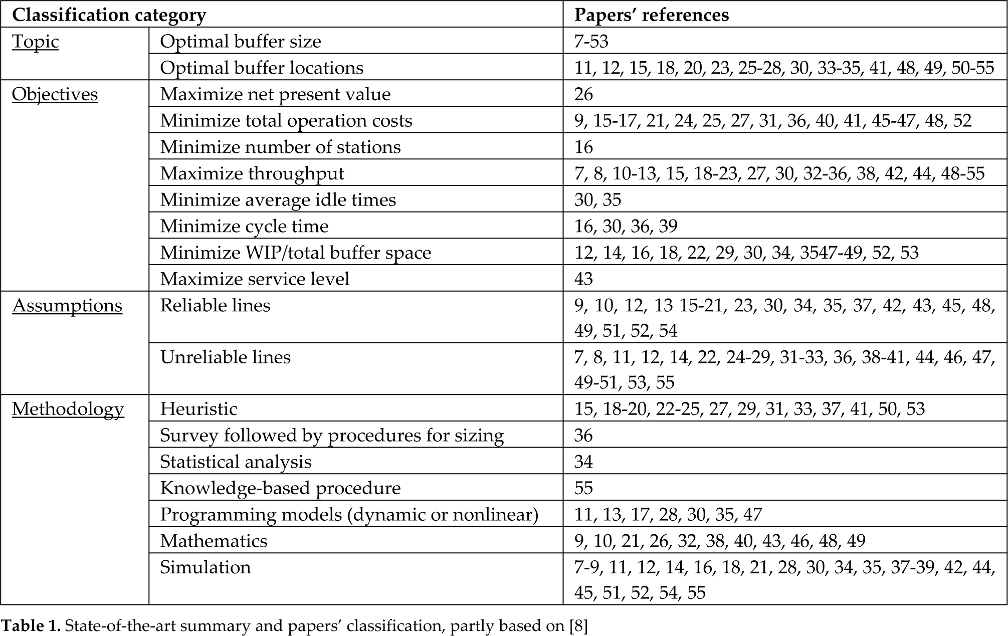
Following the classification system introduced by Battini, Persona and Regattieri [8], research works in that field can be further differentiated by the objectives pursued (to maximize net present value, minimize total operation costs, minimize the number of stations, maximize throughput, minimize average idle times, minimize the cycle time, minimize work in process (WIP) and the total buffer space, and maximize the service level), by the assumptions made (reliable or unreliable lines), and by the methodology adopted (generally heuristic, typical of operations research - a survey followed by procedures for sizing, mathematics and simulation). In Table 1, existing papers covering the buffer allocation and size problems are grouped according to this classification system.

Table 1.

State-of-the-art summary and papers' classification, partly based on [8]

Classification category		Papers' references
Topic	Optimal buffer size	7–53
Topic	Optimal buffer locations	11, 12, 15, 18, 20, 23, 25–28, 30, 33–35, 41, 48, 49, 50–55
Objectives	Maximize net present value	26
	Minimize total operation costs	9, 15–17, 21, 24, 25, 27, 31, 36, 40, 41, 45–47, 48, 52
	Minimize number of stations	16
	Maximize throughput	7, 8, 10–13, 15, 18–23, 27, 30, 32–36, 38, 42, 44, 48–55
	Minimize average idle times	30, 35
	Minimize cycle time	16, 30, 36, 39
	Minimize WIP/total buffer space	12, 14, 16, 18, 22, 29, 30, 34, 3547–49, 52, 53
	Maximize service level	43
Assumptions	Reliable lines	9, 10, 12, 13 15–21, 23, 30, 34, 35, 37, 42, 43, 45, 48, 49, 51, 52, 54
Assumptions	Unreliable lines	7, 8, 11, 12, 14, 22, 24–29, 31–33, 36, 38–41, 44, 46, 47, 49–51, 53, 55
Methodology	Heuristic	15, 18–20, 22–25, 27, 29, 31, 33, 37, 41, 50, 53
	Survey followed by procedures for sizing	36
	Statistical analysis	34
	Knowledge–based procedure	55
	Programming models (dynamic or nonlinear)	11, 13, 17, 28, 30, 35, 47
	Mathematics	9, 10, 21, 26, 32, 38, 40, 43, 46, 48, 49
	Simulation	7–9, 11, 12, 14, 16, 18, 21, 28, 30, 34, 35, 37–39, 42, 44, 45, 51, 52, 54, 55

In the most recent papers (published from 2008 to 2013, on which the present authors have focused since a detailed and complete literature review of the previous works is provided in [8]), researchers' efforts have concentrated on developing and applying new algorithms [47, 48] and approaches [53] to solve the introduced problems, on analysing different categories of production lines (such as closed serial production lines [51] or remanufacturing systems [49]), and, most of all, on creating user-friendly tools that practitioners would be able to easily apply to existing lines [50, 52], all in order to facilitate the penetration of developed methodologies in industrial operations practices. Of particular interest seems to be the innovative work of Demir, Tunali, Türsel Eliiyi and Løkketangen [53], who developed a two loop-based integrated approach using search algorithms to maximize the throughput rate of the line with a minimum total buffer size, and of Tsadiras, Papadopoulos and O'Kelly [52], who created an artificial neural network-based tool to solve the BAP and to assist production line designers in making related decisions.

A proper framework for the diffusion of these methodologies at a practical level, as already stated in 2009 by Battini, Persona and Regattieri [8], is still partially missing, as approaches based on mathematics are generally too complicated, while those based on simulation take too long to implement, and are difficult to standardize and simplify [7,8]. Furthermore, existing approaches are often not properly related to industrial standard performance parameters (such as OEE or availability, even if most of them consider them to be critical issues [8]), which would enable the relating of ineffective buffer sizing to productivity losses, and hence make it easier to quantify and compare the costs and benefits of various solutions [7].

For all of these reasons, an analytic relation to easily couple the buffer size to lines' performance has been developed and validated, and it is subsequently recalled - by the authors - in order to allow practitioners to immediately quantify the inter-operational buffer capacity needed [7].

3. Optimal Buffer Sizing - Proposed Model

The proposed model follows the aforementioned paradigm of BDFA [7, 8], aimed at individuating the maximum buffer size that facilitates the maximum OEE for automated production flow lines, taking into account different performance parameters as well as inventory costs. The proposed model is analytical, to be easy to implement in practice, but based on simulation so as to ensure the robustness of the solution and a reduced difference with the mathematical optimum (error).

It is generally true that the bigger is the buffer, the higher is the OEE, but once that the maximum buffer size is reached, no further OEE improvements will then be obtained. In addition, considering a synchronous flow shop line with “n” stations in series - when inter-operational buffers are null - the efficiency of the whole system will be the product of each individual station's productivity (and the performance of each station will depend on the previous' one, i.e., they are in complete dependence), while when inter-operational buffers are properly sized, the productivity of the line will coincide with the bottleneck's productivity (complete independence) [7].

The model is therefore meant to relate the line productivity and the buffer size, taking into account the effect of cycle time variability and minor stoppages (frequently verified in highly automated production lines because of stuck or blocked materials and work-pieces, as well as other breakdowns of short duration [8]).

The size of the buffer will therefore be calculated based on typical performance parameters, such as the mean time between failures (MTBF) and the mean time to repair (MTTR).

In order to obtain the presented easy-to-implement analytical relation, it has been necessary to mathematically model the problem and to perform a series of simulations, whose results have been validated and then observed and analysed to simplify and approximate the existing relations. The reference configuration used to perform the simulations consists of two consecutive work stations separated by a buffer (see Figure 1), as results are easily extendable to more complex lines.

Figure 1.

Model configuration [7]

Only the principal assumptions forming the basis of the validated model, and the validity ranges and analytical results, will be briefly recalled, referring to previous works for a more complete dissertation on the performance and validation of both the simulation and analytical results [7].

3.1 Assumptions and validity ranges

The model proposed relies on several assumptions, mainly regarding the line characterization.

First of all, in automated production lines, different stations are usually balanced – hence, their ideal process times (Ti) can be considered to be equal and variable within the following range, the bounds of which are expressed in minutes: [0,01667; 0,25].

In addition, not all of the productivity losses - here classified according to the OEE general notation [56] - have been considered:

Loss of quality due to the presence of defects in pieces can usually be neglected in flow shop production lines (also considering that they influence the size of buffers only in correspondence with control stations);

Loss of Performance can partly be consolidated with loss of availability (as far as minor stoppages are considered, it being possible to treat them just like stations' stops - see next bullet), and partly (referring to cycle time slowdown) modelled according to the queue theory principle [57]. In practice, according to the authors' consideration of Kingman's equation [58] and given the experienced cycle time variability ranges in flow shop lines, it is possible to model cycle time variability with an exponential, obtaining an upper bound for the size of the buffers and gaining robustness [7]. The performance index is meant to vary within the range [0,8; 0,99], and it can be different from one station to the next within the same line.

Loss of availability is made up of failures and setup (as setup and major failures usually imply the stoppage of the entire production line, only minor failures have been considered, when the buffers allow the avoidance of the nullification of production while doing maintenance on a single station). Such loss is represented through various indexes: the MTTR (ranging from 0,01 to 30 minutes in automated lines), the availability index (within the range [0,8; 0,99]), and the MTBF (a direct function of availability). Both the MTTR and the MTBF are supposed to be normally distributed with a standard deviation included within the range [5%- 100%]. The MTTR of the first station can be at most equal to the second. Since the model envisages failure durations of up to 30 minutes (a relatively long time given the high speed and reliability of the automated lines considered), loss of availability has still been analysed separately from loss of performance, even if only minor failures are taken into account (as they cannot be assimilated to minor stoppages and slowdowns).

3.2 Analytical relations

The effects of cycle time variability and of minor stoppages have been analysed separately in order to better understand their influence on OEE and buffer size B.

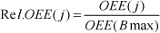
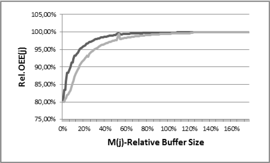
To more easily take into account the influence of cycle time variability, it has been necessary to express the performance of the production line as a percentage of the maximum achievable OEE value, i.e., the ratio between the maximum performance in terms of OEE corresponding to a selected buffer size “j” (OEE(j)) and the ideal OEE (OEE(Bmax), when the buffer's size is the maximum, completely decoupling the two work stations). The parameter Rel.OEE(j) has therefore been introduced:

Re l . O E E (j) = \frac{O E E (j)}{O E E (B max)}

(1)

When the selected buffer size is null, Rel.OEE(0) is equal to:

\frac{O E E (1) * O E E (2)}{min (O E E (1); O E E (2))}

(2)

where OEE(1) and OEE(2) are, respectively, the OEE value of the first and the second work stations when the buffer size is null.

While input parameters vary within the validity ranges, the simulation results clearly show that an ineffective buffer size dramatically affects the performance of the line, which is improved by the buffer size increase but only until an opportune value is reached (see Figure 2, where the maximum curve represents the configuration with the lowest difference in the performance index between the two stations, while the minimum is that with the highest).

Figure 2.

Rel.OEE vs. buffer size in systems affected by variability due to speed losses [7]

The effect of minor stoppages is next considered.

The ratio MTTR(2)/(Ti/P(1)) represents the maximum amount of material produced by the first station while a failure occurs in the second one, while the ratio MTTR(1)/(Ti/P(2)) represents the maximum amount of material to be stored so as not to affect the second station when a failure occurs in the first one. The maximum between these two ratios is approximately equal to the buffer size, not taking into account the effect of MTTR and MTBF variability, as well as the effect of cycle time speed losses and the moment at which the first failure occurs (which are instead taken into account by simulations). The buffer size B is therefore expressible as a percentage M of that quantity, i.e.:

M (j) = \frac{B (j)}{max (\frac{M T T R (1)}{\frac{Ti}{P (2)}}; \frac{M T T R (2)}{\frac{Ti}{P (1)}})})

(3)

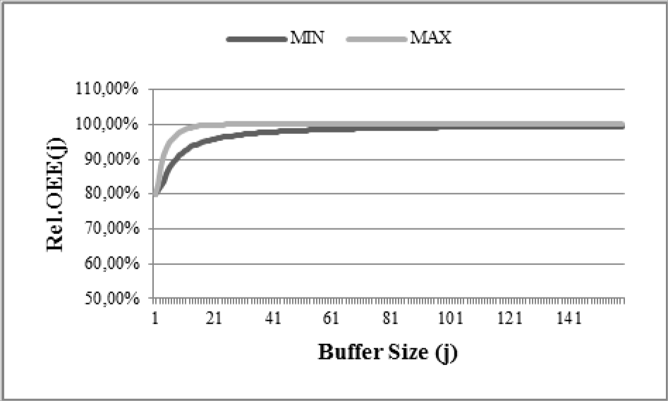
Once defined as the availability value, the Rel.OEE trends obtained by making M(j) (thus MTTR) vary, are represented in Figure 3 (the maximum curve represents the configuration with the lowest ideal cycle time, while the minimum curve is the one with the highest).

Figure 3.

Relative OEE, depending on the relative buffer size M(j) for a defined value of availability [7]

By the analysis of Figure 2 and 3, it is clear how uncertainness in performance and availability leads to buffers oversizing, but this can be prevented in most cases through a proper study of the frequency of times that it is really necessary, markedly reducing costs.

The dependency of Rel.OEE on M(j) turns out to be highly regular, allowing it to be formulated in an analytical way. Considering that, in limit configurations (when OEE(1), OEE(2) or both tend to 100%), the Rel.OEE of the production line is independent from the buffer size, the analytic expression extrapolated by the authors according to the simulation results [7] is the following:

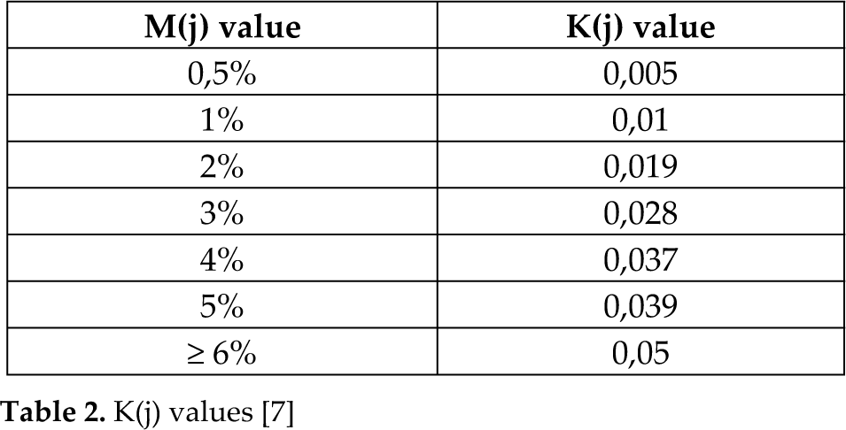
\frac{Re l . O E E (j)}{(1 - Re l . O E E (0))} = \frac{K (j) * (1 - M (j))}{M (j)}

(4)

where Rel.OEE(0) is the relative value of OEE when the buffer size is zero (the complete dependence case), K(j) is an experimental coefficient that takes into account that the obtained curve is not a real hyperbole (its values, derived from several observations into the defined range, but applicable to out-of-range values after further validation and simulations, are reported in Table 2), and M(j) is included within the range [0,05%; 100%]; as for lower values, the buffer can be considered null, while for higher values the increase in OEE is negligible.

Table 2.

K(j) values [7]

M(j) value	K(j) value
0,5%	0,005
1%	0,01
2%	0,019
3%	0,028
4%	0,037
5%	0,039
≥ 6%	0,05

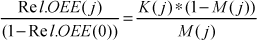
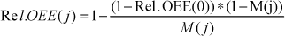
Relation 4 can be also rewritten as follows in order to make Re.OEE(j) explicit:

Re l . O E E (j) = 1 - \frac{(1 - Rel . OEE (0) * (1 - M (j)))}{M (j)}

(5)

The analytic relation has then been validated through numerical comparison with simulation results, obtaining statistically satisfying outcomes (Figure 4 reports the R-square index values between the analytic and simulation results).

Figure 4.

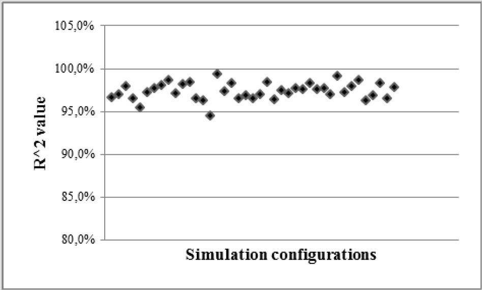
R-square index between the analytic values and the simulation results [7]

4. Pharmaceutical Packaging Line Description

The pharmaceutical packaging line that has been the object of the case study application deals with the labelling of bottles and phials and their packing and packaging. The model proposed has been applied to an existing line to validate and verify - and possibly reconsider - its first sizing, as the company, in the manner of a lean project, had fixed the objective to reduce the buffer sizes on the line as much as possible (i.e., without decreasing its efficiency). Moreover, the current huge buffer size (300 units) entailed several difficulties in its management, as bottles used to smash after being pressed against each other, stopping the line. The company's expressed need to reduce the size of this specific buffer is therefore due to both the fact that it contains value-added products, as it is positioned at the very end of the whole production line (therefore, it receives almost finite products, and its significant dimensions entail quite a large WIP), and to the fact that there are technical difficulties to deal with the current large size.

Single bottles are loaded onto an initial buffer made up of a rotating plate. The main function of this buffer is to reduce the number of times the operator is required to load bottles onto the station. A foldable orthogonal lever hinged at its centre is used to block the system when it is overloaded.

The bottles are then pushed into a guided channel (whose length is equal to a quarter of the rotating plate), leading them to an initial conveyor belt that belongs to work station A (the labeller). Always standing on the belt, the bottles are supplied with an adhesive label and then go through an optical scanner to be checked; afterwards, they are carried to the actual inter-operational buffer (totally similar to the initial one, with the lever to stop both the belt and work station A when the saturation level is reached), gathered and then sent to work station B.

Once entered into work station B, the bottles are laid down on a second partitioned conveyor belt, where a phial coming from a separated screw feeder is placed next to each bottle. Afterwards, the coupled bottle and phial are packed together (adding a patient information slip), and then “n” single packs are gathered in a bigger package (for simplicity, all of these activity have been associated with the work station B, being rigidly connected).

In Figure 5, a schematic representation of the system described is provided.

Figure 5.

Schematic representation of the pharmaceutical packaging line described

4.1 Data gathering

The data to be collected on the packaging line were:

The ideal throughput achievable in ideal conditions (without considering inefficiencies).

Availability and MTTR.

The current inter-operational buffer size.

The ideal throughput has been measured manually, clocking the time interval in which a certain number of products were pushed out of the work stations. The time interval has been chosen as short enough not to observe any stoppage, and defects were not considered (trying to reproduce ideal conditions).

The uptime and downtime periods were estimated to calculate the availability and the MTTR, considering that:

The labelling station does not often present failures but bottles used to fall off the conveyor band, causing the stoppage of the whole station.

Bottles rejected by the control station after the labeller have been considered within the downtime to avoid adding a quality parameter (that was possible thanks to their very little number).

Some more stoppages of the station A have been caused by the excessive fulfilment of the initial buffer, but they have not been counted as a downtime, being a physiological and dynamic phenomenon.

Work station B does not often present failures either, but its stoppages are often caused by bottles in a wrong position at its entrance and stoppages of the packing and packaging stations, that are rigidly connected.

Eventually, the current buffer's size was an already known parameter that has been drawn from existing databases.

The data collected and their values are summarized in Table 3.

Table 3.

Data collection

Parameter	Symbol	Unit	Value
Ideal throughput station A	V(a)	pieces/minute	75
Ideal throughput station B	V(b)	pieces/minute	60
Availability station A	A(a)	%	90,90
Availability station B	A(b)	%	92,86
Mean time to repair station A	MTTR(a)	minutes	1,5
Mean time to repair station B	MTTR(b)	minutes	2
MTTR standard deviation (A and B)	Σ	%	20
Current capacitybuffer	CCB	Units	300

The ideal process times (calculated as the inverse ratios of the ideal throughputs) are therefore 0.01334 minutes for station A and 0.01667 minutes for station B; hence, the highest one (Bin that case) will be considered as the proxy of the process time for the entire line.

5. Results of the Case Study Application

The results of the application of the previously presented analytic relations for the described production line are presented in Figures 6 and 7.

Figure 6.

Relative OEE and OEE depending on buffer size

Figure 7.

Relative OEE depending on relative buffer size

The graphs above show how the existing system is oversized. In fact, to reach complete independence between the two stations, a buffer of 110 units is sufficient, given that OEE increases negligibly above this line.

Even adding a safety margin of 20–30% for not having considered some of the failures' causes, the current buffer of 300 units appears to be a waste of space, resources and WIP, as it would be possible to reduce it of the 50%, thus decreasing costs without giving away any benefit.

The results have then been empirically tested, making the line work with a reduced buffer capacity of 150 units for a defined time period. During this period, no stoppages, slowdowns or malfunctions have been detected that could be attributed to the buffer capacity reduction, while the OEE value was not subjected to any relevant variations. The new buffer size has therefore been adopted by the company, and the reduction objective has been pursued. Eventually, the company was able to begin a study to individuate and correctly size additional inter-operational buffers from the design phase to increase the OEE of the line.

6. Conclusions and Future Developments

The application of the presented buffer sizing methodology to a real pharmaceutical packaging line has led to a buffer size reduction of about 50% in an extremely simple, fast and effective way, allowing for decreasing costs and space utilization while maintaining all buffer-related benefits.

The presented practical application has therefore confirmed the effectiveness of the buffer sizing method and its applicability to the pharmaceutical industry, highlighting its main advantages: the simplification of the buffer design phase, the optimization of spaces and work in process, with a considerable reduction in costs (a consequence that turns out to be much more critical when dealing with valuable products).

One further advantage that the methodology introduces has not yet been completely explored, namely the simplification of the buffer optimization phase. In fact, having applied a methodological approach for buffer sizing, it will be possible to immediately understand where to act during operation and maintenance in case the system does not comply with the expected standards and performance levels (for example, in case the production line undergoes structural changes or, as in the presented case study, in case technical problems in managing an overestimated buffer size arise).

Future developments of this research will include the analysis of more case studies in order to further verify the methodology's effectiveness, and the application to undersized buffers, aiming at restoring an appropriate OEE value, and to the buffer design phase (which is the phase the presented model has been developed for). Creating even more user-friendly tools for buffer sizing will also be necessary, aiming to make it a very simple application for practitioners. Currently, the authors have identified in a tabular methodology the natural expansion of the analytical method, working on charts that implement the analytical relations recalled in this paper, fixing some of the input values and letting others vary with established steps, making the buffer design phase much simpler and faster, even if a little bit less precise (a problem not really affecting industrial applications, which used to be naturally approximate).

References

Ahmed

Benson

(1999) Appendix 1. In Benchmarking in the Process Industries. Institute of Chemical Engineers.

Benson

(2005) Patient heal thyself. Drugs Discovery Today 10(3): 159–161.

Keeling

Lösch

Schrader

(2010) Outlook on pharma operations. McKinsey&Company. http://www.google.it/url?sa=t&rct=j&q=&esrc=s&source=web&cd=2&ved=0CDUQFjAB&url=http%3A%2F%2Fwww.mckinsey.com%2Fclient_service%2Foperations%2Fpeople%2F∼%2Fmedia%2F6E8A4839BDF44666A6159109FED63521.ashx&ei=9RM8U_CIIceGywPXh4GYAg&usg=AFQjCNGb_9GoE_PLvb8a_R325km4xr6BpA&bvm=bv.63934634,d.bGQ&cad=rja. Accessed on 02 Apr 2014.

Bhar

(2011) Using OEE for Packaging Line Improvement. ISPE Knowledge Brief.https://www.google.it/url?sa=t&rct=j&q=&esrc=s&source=web&cd=1&ved=0CC4QFjAA&url=https%3A%2F%2Fwww.ispe.org%2Fknowledge-briefs%2Fusingoee-for-packaging-line-improvement.pdf&ei=PhU8U-2qCceGywPXh4GYAg&usg=AFQjCNGiOZD6uCxJim_J8Ptij4mEvGS2Bg&bvm=bv.63934634,d.bGQ&cad=rja. Accessed on 02 Apr 2014.

Stambaugh

(n.d.) Pharmaceutical Packagers discover Efficiency gains from other industries. Hartness International. http://www.packagingconnections.com/downloads/download225.pdf. Accessed on 02 Apr 2014.

ISPE (2011) Overall Equipment Effectiveness (OEE) and Its Application in Pharma/Biopharma Manufacturing. Part 2 of 4 – OEE State of the Art in the Pharma Industry. http://www.google.it/url?sa=t&rct=j&q=&esrc=s&source=web&cd=1&ved=0CC4QFjAA&url=http%3A%2F%2Fwww.ispe.org%2Fomcop%2Foee-oct2010-oeebasic-philosophy-definitions-part1-4.pdf&ei=HA88U76bN8a0yAOqvoHQCA&usg=AFQjCNEHpV9CcLDQB0dpuX4zzM7U6YDkhQ&bvm=bv.63934634,d.bGQ. Accessed 2013 Apr 02.

Cesarotti

Giuiusa

Introna

(2011) Increasing availability of production flow lines through optimal buffer sizing: a simulative study. Proceedings of the 23rd European Modeling and Simulation Symposium, September 12–14 2011, Rome, Italy.

Battini

Persona

Regattieri

(2009) Buffer size design linked to reliability performance: A simulative study. Computers & Industrial Engineering 56: 1633–1641.

Anderson

Moodie

(1969) Optimal buffer storage capacity in production line systems. International Journal of Production 3(3).

10.

Hillier

Boiling

(1977) On the optimal allocation of work in symmetrically unbalanced production line

11.

Chow

(1987) Buffer capacity analysis for sequential production lines with variable process times. International Journal of Production Research 25(8): 1183–1196.

12.

Conway

Maxwell

McClain

Thomas

(1988) The role of work-in-process inventory in serial production lines. Operations Research 36(2): 229–241.

13.

Pourbabai

(1989) Optimal selection of the local storage sizes of an assembly system. International Journal of Production Research 27(9), 1625–1636.

14.

Szendrovits

Miltenburg

Goldstein

(1990) Optimizing total safety inventory for large transfer lines. Omega 18(3): 299–313.

15.

Hiller

(1993) Some data for applying the bowl phenomenon to large production line systems. International Journal of Production Research 31(4):811–822.

16.

Malakooti

(1994) Assembly line balancing with buffers by multiple criteria optimization. International Journal of Production Research 32(9): 2159–2178.

17.

Lee

Young

(1997) Price-based buffer sizing in assembly systems. Computers and Industrial Engineering 33(3–4): 709–712.

18.

Lutz

Davis

Sun

(1998) Determining buffer location and size in production line using tabu search. European Journal of Operational Research 106: 301–316.

19.

Powell

Pyke

(1998) Buffering unbalanced assembly systems. IIE Transactions 30: 55–65.

20.

Papadopoulos

Vidalis

(1998) Optimal buffer storage allocation in balanced reliable production lines. International Transactions in Operational Research 5(4): 325–339.

21.

Spinellis

Papadopoulos

(1999) Production line buffer allocation: Genetic algorithms versus simulated annealing. Second International Aegan conference on the analysis and modelling of manufacturing systems: 12–101.

22.

Gershwin

Schor

(2000) Efficient algorithms for buffer space allocation. Annals of Operations Research 93: 117–144.

23.

Hillier

(2000) Characterizing the optimal allocation of storage space in production line with variable processing times. IIE Transactions 32: 1–8.

24.

Jeong

Kim

(2000) Heuristics for selecting machines and determining buffer capacity in assembly systems. Computers and Industrial Engineering 38(3): 341–360.

25.

Shine-Der

(2000) Buffer sizing in complex cellular manufacturing system. International Journal of Systems Science 1(8): 937–948.

26.

Helber

(2001) Cash-flow-oriented buffer allocation in stochastic flow lines. International Journal of Production Research 39(14): 3061–3083.

27.

Papadopoulos

Vidalis

(2001) A heuristic algorithm for the buffer allocation in unreliable unbalanced production lines. Computers and Industrial Engineering 41: 261–277.

28.

Sörensen

Janssens

(2001) Buffer allocation and required availability in a transfer line with unreliable machines. International Journal of Production Economics 74: 163–173.

29.

Sooyoung

Haeng-Ju

(2001) Allocation of buffer capacity to minimize average work-in-process. Production Planning and Control 12(7): 706–716.

30.

Huang

Chang

Chou

(2002) Buffer allocation in flow-shop-type production systems with general arrival and service patterns. Computers and Operations Research 29: 103–121.

31.

Shin-Der

Sui-hwa

(2002) Buffer sizing in manufacturing production system with complex routing. International Journal of Computer Integrated Manufacturing 15(5): 450–452.

32.

Enginarlar

Jingshan

Meerkov

Zhang

(2002) Buffer capacity for accommodating machine downtime in serial production lines. International Journal of Production Research 38.

33.

Leyuan

Shuli

(2003) Optimal buffer allocation in production line. IIE Transactions 35(1): 1–100.

34.

Chiadamrong

Limpasontiong

(2003) Using storage buffer to improve unbalanced asynchronous production flow line's performance. International Journal of Manufacturing Technology and Management 5(1/2): 149–161.

35.

Hemachandra

Eedupunganti

(2003) Performance analysis and buffer allocations in some open assembly systems. Computers and Operations Research 30: 695–704.

36.

Tempelmeier

(2003) Practical considerations in the optimization of flow production systems. International Journal of Production Research 41(1): 149–170.

37.

Yamada

Matsui

(2003) A management design approach to assembly line systems. International Journal of Production Economics 84: 193–204.

38.

Gutowski

(2005) Inventory buffer size. Working paper. Available from http://web.mit.edu.

39.

Louw

Page

(2004) Queuing network analysis approach for estimating the sizes of the time buffers in Theory of Constraints-controlled production systems. International Journal of Production Research 42(6): 1207–1226.

40.

Zequeira

Prida

Valdes

(2004) Optimal buffer inventory and preventive maintenance for an imperfect production process. International Journal of Production Research 42(5): 959–974.

41.

Aksoy

Gupta

(2005) Buffer allocation plan for remanufacturing cell. Computers and Industrial Engineering 48: 657–677.

42.

Vidalis

Papadopoulos

Heavey

(2005) On the workload and ‘phase load’ allocation problems of short reliable production line with finite buffers. Computers and Industrial Engineering 48: 825–837.

43.

Van Nieuwenhuyse

Vandaele

Rajaram

Karmakar

(2006) Buffer sizing in multi-product multi-reactor batch processes: Impact of allocation and campaign sizing policies. European Journal of Operational Research.

44.

Ribeiro

Silveira

Quassim

(2007) Joint optimisation of maintenance and buffer size in a manufacturing system. European Journal of Operational Research 176(1): 405–413.

45.

Yamamoto

Qudeiri

Marui

(2007) Definition of FTL with bypass line and its simulator for buffer size decision. International Journal of Production Economics.

46.

Zequeira

Valdes

Berenguer

(2007) Optimal buffer inventory and opportunistic preventive maintenance under random production capacity availability. International Journal of Production Economics 54: 98–99.

47.

Shi

Gershwin

(2009) An efficient buffer design algorithm for production line profit maximization. International Journal of Production Economics 122: 725–740.

48.

Massim

Yalaoui

Amodeo

Chatelet

Zeblah

(2010) Efficient combined immune-decomposition algorithm for optimal buffer allocation in production lines for throughput and profit maximization. Computers and Operations Research 37: 611–620.

49.

Aksoy

Gupta

(2010) Near optimal buffer allocation in remanufacturing systems with N-policy. Computers and Industrial Engineering 59: 496–508.

50.

Demir

Tunali

Eliiyi

D Türsel

(2012) An adaptive tabu search approach for buffer allocation problem in unreliable non-homogenous production lines. Computers and Operations Research 39: 1477–1486.

51.

Staley

Kim

(2012) Experimental results for the allocation of buffers in closed serial production lines. International Journal of Production Economics 137: 284–291.

52.

Tsadiras

Papadopoulos

O'Kelly

MEJ

(2013) An artificial neural network based decision support system for solving the buffer allocation problem in reliable production lines. Computers and Industrial Engineering 66: 1150–1162.

53.

Demir

Tunali

Eliiyi

D Türsel

Løkketangen

(2013) Two approaches for solving the buffer allocation problem in unreliable production lines. Computers and Operations Research 40: 2556–2563.

54.

Powell

(1994) Buffer allocation in unbalanced three-station serial lines. International Journal of Production Research 32(9): 2201–2217.

55.

Vouros

Papadopoulos

(1998) Buffer allocation in unreliable production lines using a knowledge based system. Computers and Operations Research 25(12): 1055–1067.

56.

Huangt

Dismukes

Shi

Razzak

Bodhale

Robinson

(2003) Manufacturing productivity improvement using effectiveness metrics and simulation analysis. International Journal of Production Research 41(3): 513–527.

57.

Papadopoulos

Heavey

(1996) Queuing theory in manufacturing systems analysis and design: A classification of models for production and transfer lines. European Journal of Operational Research 92(1): 1–27.

58.

Kingman

(1966) On the algebra of queues. London: Methuen.

Buffer Size Design in Pharmaceutical Packaging Lines: An Analytical Methodology Proposal and Case Study

Abstract

Keywords

1. Introduction

2. The State-of-the Art of the Buffer Design Problem

3. Optimal Buffer Sizing - Proposed Model

3.1 Assumptions and validity ranges

3.2 Analytical relations

4. Pharmaceutical Packaging Line Description

4.1 Data gathering

5. Results of the Case Study Application

6. Conclusions and Future Developments

References