
Abstract
This paper proposes a framework, namely adaptive iterative learning control (AILC), which is used in the control of a microelectromechanical system (MEMS) gyroscope, to realize high-precision trajectory tracking control. According to the characteristics of the MEMS gyroscope's model, the proposed AILC algorithm includes an adaptive law of parametric estimation and an iteration control law, which is updated in the iterative domain without any prior knowledge of MEMS gyroscopes. The convergence of the method is proven by a Lyapunov-like approach, which shows that the designed controller can guarantee the stability of the system and make the output tracking errors to converge completely to zero while the iteration index tends to infinity. By comparing AILC and traditional PD-ILC, the simulation results demonstrate the effectiveness of AILC and its robustness against external random disturbance.
Keywords
1. Introduction
MEMS gyroscopes could provide high performance angular-rate measurements leading to a wide range of applications, including navigation and guidance systems, automotive safety systems and consumer electronics. Extensive research efforts towards vibratory MEMS gyroscope -, which utilize vibrating elements to induce and detect Coriolis forces − have led to several innovative gyroscope fabrication and integration approaches and detection techniques. However, achieving robustness against fabrication variations and environmental fluctuations remains one of the greatest challenges in the commercialization and high-volume production of MEMS vibratory gyroscopes [1]. Moreover, MEMS gyroscopes belong to MIMO systems, which have parameter uncertainties and are vulnerable to external environmental influences. As a consequence, it is necessary to solve these problems by utilizing advanced control technologies, such as adaptive control, sliding mode variable control, adaptive sliding mode control, adaptive force-balancing control and fuzzy control. Paper [2] developed a sliding mode control for a MEMS gyroscope system. An adaptive controller was presented to drive both axes of vibration and control the entire operation of the gyroscope [3]. In reference [4], the SMC strategy was incorporated into an adaptive control for the vibration of a MEMS gyroscope. Paper [5] extended the method mentioned in [3] to three-axis MEMS gyroscopes. The adaptive force-balancing control proposed in [6] can identify major fabrication imperfections. In [7], an adaptive fuzzy compensator was designed to compensate dead-zone non-linearities for MEMS gyroscopes.
In 1984, Arimoto et al. [8] put forward the explicit formulation of an iterative learning control (ILC) algorithm with rigorous convergence analysis based on the previous research work of Uchiyama. After more than three decades of development, the ILC algorithm has become a branch of intelligent control with a well-established mathematical description and stability proof which can handle nonlinear and strong coupling systems in a very simple way and at low cost [9,10]. Currently, the ILC has made tremendous progress in terms of the learning law, convergence, robustness, learning speed and application, and it has been used in industrial robots, rotary systems, heat treatment, and chemical production processes, etc. [9]. Adaptive ILC, integrating the merits of adaptive control and ILC based on Lyapunov stability theory, is very popular and frequently attracts the attention of researchers. Paper [11] proposed an adaptive learning scheme for uncertain robot systems on the basis of parameter linearization; paper [12] provided not only an AILC method for industrial robots but also the results of experiments; in paper [13,14], the authors used standard Lyapunov stability theory to design an AILC algorithm, while [15–18] exploited a Lyapunov-like theory to prove the convergence of AILC. In paper [17], three AILC schemes were put forward for rigid robot manipulators, and the subsequent study of AILC was presented in paper [18], describing a unified AILC framework for uncertain nonlinear systems and interpreting the advantages and disadvantages of pure time-domain adaptation, pure iteration-domain adaptation and 2-D adaptation. In the last five years, there have been two main trends in AILC. The first one is AILC for discrete-time systems, namely the fusion of discrete-time adaptive control theory and ILC [19–21], which extends the application range of AILC; the second trend is the combination of AILC with other intelligent control theories [22,23] (fuzzy control, neural network control, etc.), which may assist in designing better controllers in achieving the desired performance, such as the relaxation of resetting conditions or alignment conditions, and robustness against external disturbances.
However, ILC has not been investigated for a MEMS gyroscope in the literature. Hence, an ILC strategy for MEMS vibratory gyroscopes is proposed in this paper. The research motivation of ILC is that some systems which run repetitive tasks in fixed time-intervals can improve their performance from previous operational experience - that is to say that systems can reduce tracking errors by incorporating past control information, such as tracking errors and control input signals. Due to the inherent characteristics of AILC, the approach requires less prior knowledge of process or systems at the stage of controller design than other methods, so it can deal with problems of unknown parameters or parametric uncertainties, especially for nonlinear, strong coupling dynamic systems. The main characteristics of the proposed AILC with their application to a MEMS gyroscope are highlighted as follows:
An AILC algorithm, including an adaptive law of parametric estimation and an iteration control law, is designed to improve the robustness of the control system. It integrates the advantages of adaptive control and ILC, and guarantees that the tracking error can converge to zero. The AILC design approach is used to drive the trajectory tracking errors to converge to zero rapidly.
An AILC is incorporated into the MEMS gyroscope to improve the tracking performance and strengthen the robustness of the control system. The convergence of the proposed algorithm using a Lyapunov-like theory can be established. This control scheme consists of conventional PD feedback control, unknown parameters and tracking errors of iteration.
Simulation studies verify the robustness of the algorithm using random disturbance signals instead of repetitive disturbance signals in every iterative control. By comparing AILC and traditional PD-ILC, the simulation results show the effectiveness of AILC and its robustness against external random disturbance
This paper is organized as follows. In Section 2, the dynamics of the MEMS gyroscope are described. In Section 3, the adaptive iterative learning controller is derived and the stability of the designed control systems is proved by Lyapunov's stability theory. Simulation results are presented in Section 4. Finally, conclusions are provided in Section 5.
2. Dynamics of the MEMS gyroscope
A typical MEMS vibratory gyroscope includes a proof mass suspended by spring beams, electrostatic actuations and sensing mechanisms for forcing an oscillatory motion and sensing the position and velocity of the proof mass. A z-axis MEMS gyroscope is depicted in Figure 1. The dynamics of a MEMS gyroscope are derived from Newton's law in the rotating frame.

A simplified model of a MEMS z-axis gyroscope
As we know, Newton's law in the rotating frame becomes:

where Fr is the total applied force to the proof mass in the gyro frame, Fphy is the total physical force to the proof mass in the inertial frame, Fcentri is the centrifugal force, FColis is the Coriolis force, FEuler is the Euler force, and ar is the acceleration of the proof mass with respect to the gyro frame.
Assuming that the gyroscope is almost rotating at a constant angular velocity Ω over a sufficiently long time interval, that the stiffness of the spring in the z direction is much larger than that in the x,y directions, and the motion of the proof mass is constrained only along the x − y plane, we have Ω x = Ω = 0.
In Equation (1), the expression for the Euler force reduces to
For another, the expression for centrifugal force reduces to Fcentri = −mΩ×(Ω×rr). Under a typical assumption Ω x = Ω y = 0, and the centrifugal forces along the x-axis and the y-axis can be expressed as Fcentri–x = −mΩ z 2x and Fcentri–y = −mΩ z 2y, where x, y are displacements of the proof mass along the x-axis and the y-axis. Considering the fact that Fcentri–x and Fcentri–y are very small - usually no more than one thousandth of other forces − as such they can be ignored.
Similarly, the expression for the Coriolis force reduces to FColis = −2mΩ × vr, where vr is the velocity vector relative to the rotating gyroscope frame. According to the principle of Coriolis force, the Coriolis forces along the x-axis and the y-axis can be expressed as FColis–x = 2mΩ z ẏ and FColis–y = −2mΩ z ẋ, where ẋ, ẏ are velocities of the proof mass along the x-axis and the y-axis.
The total physical force to the proof mass in the inertial frame Fphy mainly consists of the driving force, the spring force and the damping force. Here, we make the following statements: ux, uy are the control forces in the x,y directions; and kxx, kyy and dxx, dyy are the spring and damping coefficients of the x and y axes; kxy and dxy are the asymmetric spring and damping terms, which are mainly contributed by fabrication imperfections. Further, the total physical force in the inertial frame along the x-axis and the y-axis can be expressed as Fphy–x = ux − kxxx − kxyy − dxxẋ − dxyẏ and Fphy–y = uy − kyyy − kxyx − dyyẏ − dxyẋ.
Based on the above analysis, the dynamics of the gyroscope are simplified as follows:

Using non-dimensional time t* = ω0t, where ω0 is a natural resonance frequency about 1 KHz, then we have:

Substituting Eq. (3) into Eq. (2) and dividing both sides of (3) by m, q0, ω02 (which are a reference mass, length and natural resonance frequency, respectively), we get the form of the non-dimensional equation of motion as:
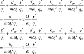
The vector-form of the MEMS gyroscope dynamics model can be written as:
where:
For concision, we define a set of new parameters as follows:
Considering the system with external disturbance, the dynamics of the MEMS gyroscope can be expressed as:

where d is an uncertain extraneous disturbance.
3. Adaptive iterative learning controller design
3.1 Control Algorithm Design
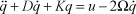
Based on the study of iterative learning control, the dynamics of the MEMS gyroscope may be expressed by:

where the nonnegative integer
We make the following assumptions prior to further discussion.
Assumption 1. The reference trajectory and its first and second time-derivative, namely qd(t), q̇
d
(t) and q̈
d
(t), as well as the disturbance dk(t), are bounded ∀t ∈ [0,T] and
Assumption 2. The resetting condition is satisfied, i.e.,
Moreover, we will also need the following properties, which are common to dynamics of MEMS gyroscope.
Kqk(t) + (D + 2Ω)q̇
k
(t) = Ψ(qk, q̇
k
)ξ, where
‖q̈ d − dk‖ < β, where β is an unknown positive parameter.
θ(t) = [ξ T (t) β] T , where θ consists of system structure parameters and β.
The tracking control problem of a MEMS gyroscope is what this paper considers, so the control target is to design a suitable control law to make the system output qk track the state of the desired trajectory qd asymptotically. The block diagram of AILC for a MEMS gyroscope is shown in Figure 2; the tracking error between the reference state and the gyroscope state comes to the adaptive iterative learning controller.

Block diagram of AILC for a MEMS gyroscope
Now, we can state the following result:
Theorem 1. If the control law (8), with the properties (i1–i3) and the parameter adaptation law (9), is applied to the nonlinear uncertain system defined by (7), then the system's tracking error can converge to zero, and all the closed-loop signals can be guaranteed bounded. Namely:

with:

where
3.2 Control Algorithm Design
The proof of the above theorem is in the next three steps. The first step is to take a positive definite Lyapunov-like composite energy function, namely Wk, and show that this sequence is non-increasing with respect to k, and hence bounded if W0 is bounded. In the second step, we show that W0(t) is bounded for all t ∈ [0,T]. Finally, we show that
Proof. Let us consider the following positive definite function as a Lyapunov function candidate:
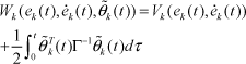
where
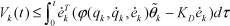
Differentiating Wk with respect to the iteration yields, we have:

We define
Substituting the above equation into (11) generates:

Note that
Hence:
where
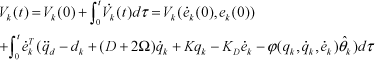
Further, we have

According to Assumption 2, ek(0) = 0 and ė k (0) = 0, such that Vk(ė k (0), ek(0)). Thus:
Considering the adaptive law


Substituting (15–17) into (12) generates:
Hence, Wk is a non-increasing sequence. Thus, if W0(t) is bounded, one can conclude that Wk is bounded.
In the next step, we will show that W0(t) is bounded for all t ∈ [0,T].
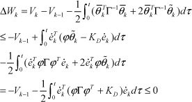
From the definition of W0(t) in (10), we have:

In fact, differentiating (15) with k = 0, we have

Since

Using Young's inequality, i.e., a2 + b2 ≥ 2ab, we have
Hence:
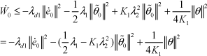
Taking
Since Wk(t) is a Lyapunov-like composite energy function and its sequence is non-increasing, we have 0 ≤ Wk(t) ≤ W0, ∀k ≥ 1. On the other hand, because W0(t) is bounded over [0,T], we can conclude that Wk(t) is bounded
Note that Wk(t) can be written as
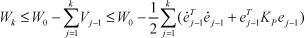
which leads to:

Eq. (24) implies that
4. Simulation example
A simulation example with a z-axis vibratory MEMS gyroscope is implemented in this section for the purpose of evaluating the performance of the AILC scheme. The parameters of the adopted MEMS gyroscope are as:
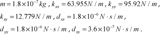
Since the general displacement range of the MEMS gyroscope in each axis is at the sub-micrometre level, it is reasonable to choose 1μm as the reference length q0. Given that the usual natural frequency of each axis of a MEMS gyroscope is within the KHz range, we thus choose ω0 as 1 KHz. The unknown angular velocity is assumed to be Ω z = 100rad / s. As such, the non-dimensional values of the MEMS gyroscope parameters are listed as follows:
ω2 x = 355.3, ω2 y = 532.9, ω xy = 70.99, dxx = 0.01, dyy = 0.01, dxy = 0.002, Ω z = 0.1. Because all the gyroscope parameters are unknown or uncertain, they are invisible to our controller.
In this simulation example, the desired motion trajectories are described by
In order to demonstrate the effectiveness of the control algorithm, a comparable investigation is accomplished between the proposed AILC and PD-type iterative learning controller (PD-ILC). The PD iterative learning controller is defined as uk(t) = uk−1(t) + Kpek(t) + KDek(t), where u−1(t) = 0 and the other parts, such as the definitions of the variables and parameters' values, are the same as the AILC algorithm. In the simulation, the iterations of these two iterative algorithms are set as five-times over the time interval [0,2s]. The simulation results are shown in Figures 3∼5.
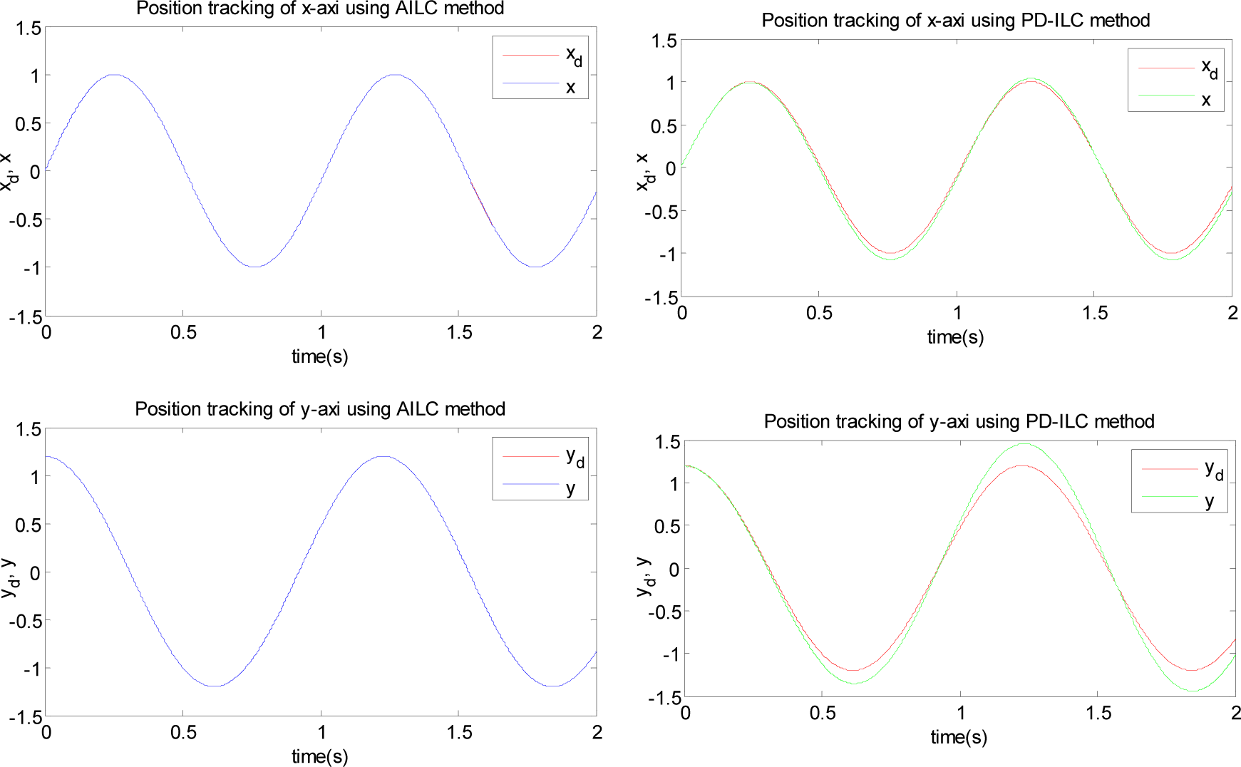
Comparison of the position tracking of the x-axis and the y-axis between AILC and PD-ILC

Maximum absolute value of the x-axis and y-axis position errors for the two methods

Comparison of the velocity tracking of the x-axis and the y-axis between the AILC and the PD-ILC
Figure 3 depicts the MEMS gyroscope along the x-axis and the y-axis position tracking trajectories between the AILC algorithm and the PD-ILC algorithm in the fifth iteration cycle. It can be observed intuitively that the actual motion trajectory of the MEMS gyroscope is consistent with the desired reference trajectory using the AILC algorithm, demonstrating that the adaptive tracking performance is satisfactory. However, the actual motion trajectory has an obvious interval from the reference trajectory when utilizing the PD-ILC algorithm.
Figure 4 describes that the maximum absolute value of the x-axis and the y-axis position errors in two methods of five iterations, where ex = max(|xd(t) − xk(t)|), ey = max(|yd(t) − yk(t)|), ∀t∈ [0,T]. From Figure 4, it can be seen that the maximum absolute value of the x-axis and the y-axis corresponding to the AILC decreases obviously in contrast with the PD-ILC.
Figure 5 and Figure 6 show the MEMS gyroscope velocity tracking trajectories and the maximum absolute value of the velocity tracking errors along the x-axis and the y-axis between two methods. The maximum absolute value of the velocity tracking errors along the x-axis and the y-axis are defined as
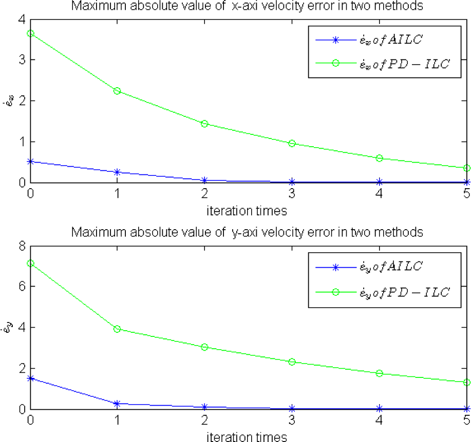
Maximum absolute value of the x-axis and y-axis velocity errors for the two methods
5. Conclusion
In this paper, we have proposed the design of a new AILC for MEMS vibratory gyroscopes under unknown model uncertainties and external disturbances. First, the dynamic model of a two-axis MEMS vibratory gyroscope is briefly introduced. Next, the AILC approach is used to drive the trajectory tracking errors to rapidly converge to zero. This control scheme consists of conventional PD feedback control, unknown parameters and the tracking error of iteration. Based on Lyapunov's stability theory, we construct a Lyapunov definite function candidate, demonstrating that the position and velocity tracking errors all converge to zero. Finally, comparative simulation results between the AILC algorithm and a PD-ILC algorithm are implemented to verify the effectiveness of the proposed AILC strategies.
Footnotes
6. Acknowledgements
The authors would like to thank the anonymous reviewers for their useful comments, which have helped to improve the quality of the manuscript. This work was supported by the National Science Foundation of China under Grant No. 61374100, the Natural Science Foundation of Jiangsu Province under Grant No. BK20131136, and the Fundamental Research Funds for the Central Universities under Grant No. 2013B101-09.