Sage Journals: Discover world-class research

Abstract

The most important feature of a Self-Reconfigurable Robot (SRR) is that it is reconfigurable and self-repairing. At the centre of these capabilities is autonomous docking. One difficulty for docking is the alignment between two robots. Current strategies overcome this by integrating a mechanical guiding device within the connecting mechanism. This increases the robustness of docking but compromises the flexibility of reconfiguration. In this paper, we present a new autonomous docking strategy that can overcome the drawbacks of current approaches. The new strategy uses a novel hook-type connecting mechanism and multi-sensory guidance. The hook-type connecting mechanism is strong and rigid for reliable physical connection between the modules. The multi-sensory docking strategy, which includes visual-sensor-guided rough positioning, Hall-sensor-guided fine positioning, and the locking between moving and target modules, guarantees robust docking without sacrificing reconfigurability. The proposed strategy is verified by docking between a worm-shaped robot and one target module, and docking among three moving robots to form a T-shaped configuration. The experimental results showed that the strategy is very effective.

Keywords

Self-reconfigurable Robot (SRR)Sensory Module Connecting Mechanism Autonomous Docking

1. Introduction

Generally speaking, a Self-Reconfigurable Robot (SRR) is a distributed robotic system consisting of multiple quasi-identical modules. What distinguishes SRR from conventional robotic system is its projected ability to self-adapt, self-reconfigure and self-repair, which can potentially make the system more robust. The problems associated with SRR are, in general, ones of transformation between different configurations. At the core of these transformations is accurate autonomous docking between modules, which allows the system to adapt to the surrounding environment or to accomplish certain tasks. The focus of this paper is the autonomous docking strategies of SRR. SRR was first proposed by Fukuda, i.e., the CEBOT [1]. Since the initial conception, many other SRR systems, including Roombot [2 –4], M-Cube [5], M-TRAN [6 –10], ModRED [11], SuperBot [12 –14] and Yamor [15 –17], to name only a few, have been developed.

Current docking algorithms are based on either infrared sensing or vision. In the infrared approach, an infrared emitter and receiver are attached to the surface of the module for alignment. Examples of such efforts include: six DOF docking algorithm [18], docking algorithm for the CONRO SRR module for realizing a snake-shaped configuration [19] and the docking algorithm for Sambot [20]. One of the drawbacks of this approach is that it does not scale well with the number of modules.

Vision can be also used to achieve accurate alignment. For example, a positioning method using a CMOS camera and three RGB LEDs has been proposed [21]. By tracking the LEDs using the camera, three-dimensional docking can be implemented. A functional module with an integrated camera is designed and the module is compatible with M-TRAN; docking is realized through visual feedback in a special docking configuration [22]. A method to control the movement of the robotic head is designed, in which colour information is used to determine the position of the object in motion [23].

One of the problems with the current docking approach is that infrared or vision alone is not enough, and require additional mechanical guiding device to accommodate positioning errors. Since the guiding components usually have male-female structures that bring extra physical constraints for connection and release between modules, they result in loss of the morphing ability in the robots. This is particularly true when a large number of modules are involved.

In this paper, we present an autonomous docking approach for SRR by combining a novel hook-type connecting mechanism and a multisensory guidance control to overcome the drawbacks of existing approaches. Our docking approach is designed for UBot SRR, but can be extended to other SRRs. In the new approach, an embedded hook-type structure is used as a connecting mechanism. The hook-type structure is hidden beneath the modular surface and brings no extra kinematic constraints to the transformation process. This increases the flexibility of reconfiguration. Precise docking is achieved by combining vision with Hall sensors, where a three-step approach that includes rough-positioning, precise positioning and docking execution is employed to eliminate the use of mechanical guidance. The system has been experimentally verified and proves to be very effective.

The rest of the paper is organized as follows: section 2 introduces the physical structure of UBot SRR which uses our novel hook-type connection mechanism. Section 3 presents our multisensory docking algorithm. Section 4 shows the experimental verification of our new docking mechanism and algorithms, and section 5 concludes the paper.

2. Physical platform of UBot

2.1 Basic module

The UBot SRR [24–25] consists of active and passive modules with the same joint motor function. Each module has four connecting surfaces and two orthogonal axes of rotation, capable of rotating from −90° to +90°. The structure of the active and passive modules and one of the physical systems is shown in Figure 1.

Figure 1.

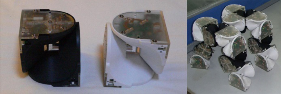
The structure of the active and passive modules and physical system

The twin-rotation mechanism determines the basic shape of the module and is the main motion mechanism of the UBot for locomotion, self-reconfiguration and operation. As shown in Figure 2, the right-angled shaft and the two L-type parts connecting to the tips of the shaft form two rotational joints which perpendicularly intersect with each other in the geometric centre of the module. Actuated by two micro-DC-geared motors, the right-angled shaft can rotate around the two L-shaped components. The control board, the driving board of the motor and the wireless communication board are fixed in the twin-rotation mechanism by bolts. Additionally, the components of the active connecting mechanism and battery are embedded in the twin-rotation mechanism.

Figure 2.

Twin-rotation mechanism

There are four holes symmetrically distributed on each of the four connecting surfaces of a module (both active and passive). The holes will line up when the surfaces of two modules are lined up. Inside each hole in an active module is a hook-type connector driven by the same motor. The holes on the passive modules are empty. The active and the passive modules can be connected via any connecting surfaces in any orientation. Four orientating magnets are installed near the hook-type connectors in both active and passive surfaces, which serve as auxiliary orientating or detected objects for the Hall sensors. The specific structural design and connecting scheme are shown in Figure 3 and Figure 4.

Figure 3.

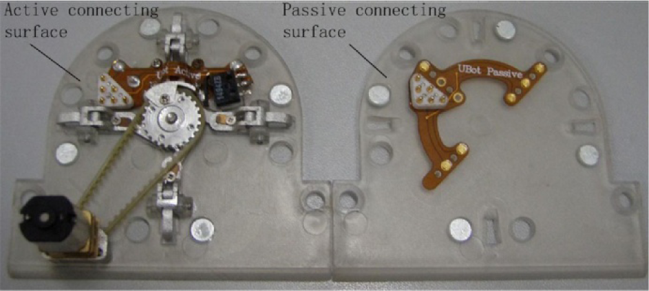
Physical structure of the docking surface

Figure 4.

The connecting scheme of hook-type connector

Figure 4 shows the process of connection. To make the connection, the sliders move outward, driven off the motor, and the drive hooks rotate around the fixed shaft via the moving shaft until the two surfaces are fastened. The connection is released by the opposite sequence. The centre timing wheel's rotation is driven by a geared motor through the timing belt. The angle of rotation is limited mechanically to the point where the centre timing wheel slightly (2°) goes beyond its maximum stretch. This is effective to prevent pull-back of the hooks without torque of the motor, and the mechanism has the function of self-locking and energy saving. Every active connecting mechanism has a position sensor which detects the connection or disconnection of the connector.

The holes in the active module and its hooking mechanism are designed to ensure that the four hooks stay beneath the modular surface except during docking. This is important to maximize flexible locomotion among large amount of modules.

2.2 Sensory module

Without mechanical aligning guidance, autonomous docking becomes challenging, especially in short distance situations. Our solution is to combine visual sensor and Hall sensor for docking guidance. The visual sensor is responsible for rough positing in long distance situations, while the Hall sensors are used for accurate positioning in short distance situations. The sensory module is designed with a cubic structure with the same dimensions as the basic module, including the hole structures, to ensure that it can dock with the active module. Inside the sensory module are four types of sensors: wireless vision sensor, accelerometer, infrared range finder and linear Hall sensor. A coloured-pinhole CCD camera is placed on one connecting surface and four linear Hall sensors are installed on the same connecting surface, matching the positions of the four orientating magnets of the active module. A fine positioning adjustment ability is achieved with the application of Hall sensors together with the existing magnets. The array of Hall sensors can detect the alignment error between the surfaces of docking and target modules. An accelerometer and infrared sensor are also included for other function development. The external structure and the internal circuit layout are illustrated in Figure 5.

Figure 5.

Structure of sensory module

Docking is implemented between a chain module group with the sensory module as the head and the active module as the target module. The module chain is set to dock with one connecting surface of the target module. We attach four, symmetrically-distributed, round=shaped yellow tags on each of the lateral target module's surfaces as characteristic features for visual recognition. With the tags, the sensory module can find the target module and calculate its relative position and orientation. A target module with the tags is shown in Figure 7.

Figure 6.

The process of extracting the target features. (a) The original image from RGB space of the visual sensor. (b) S component is used for recognition and extraction of the features from the target module, which can filter out some noisy signals coming from non-uniformly distributed lighting, decrease the influence of lighting orientation and enhance the contrast of the image. (c) Greyscale image is gained by top-hat transformation. (d) The result after image binarization: it is necessary to demonstrate black-white effect. (e) Morphological method is applied to smooth the boundaries of and filter out the noisy objects. (f) Hough transformation is used to extract the ellipse geometry features and their centre locations for further computing of the motion adjustment parameters.

Figure 7.

Docking surface recognition

3. Docking in self-reconfigurable robot

We propose a three-phased autonomous docking approach for the docking system mentioned above:

Target module recognition via wireless vision sensor and pre-positioning preparation;

Precise positioning for docking;

Docking execution and self-locking for the sensory module and the target module via hook-type connector.

3.1 Visual-sensor-guided rough positioning

3.1.1 Feature extraction

The choice of colour space is quite important for correct extraction of target features. The sensed visual information from the camera is in RGB form for the yellow tag features attached to the target module. If only one particular colour component in RGB form is retrieved, the colour information in the background will also be introduced because of the correlation between them. These disturbances will make it difficult to extract the features of the target module correctly. As a result, the RGB space could not be used directly for feature extraction. Considering the high saturation property of the yellow tags on the target module, we choose the HIS (Hue, Intensity and Saturation) colour model, where hue represents a specific tone of colour, like red, green or blue; intensity means the luminance of light and is influenced greatly by the light source; and saturation stands for the purity of the colour. We use the saturation property of the yellow tag for recognition and extraction of the features from the target module.

Based on the analysis above, the RGB colour space from the sensed visual information is converted to the form of HIS: Hue component is gained by:

H = {\begin{cases} θ, B \leq G \\ 2 π - θ, B > G \end{cases}

(1)

where θ is determined by:

θ = \arccos {\frac{(R - G) + (R + G)}{2 [{(R - G)}^{2} + (R - B) {(G - B)}^{\frac{1}{2}}]}}

(2)

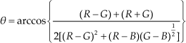
Saturation and Intensity components are:

S = 1 - \frac{3}{(R + G + B)} [\min (R, G, B)]

(3)

I = \frac{R + G + B}{3}

(4)

where the symbols R, G and B denote, respectively, the red, green and blue components from the RGB colour space. The S component is used for recognition and extraction of the features from the target module, as shown in Figure 6 (b).

To extract the circle's geometry features from the target module, first we covert the captured image from RGB space to HIS space, and obtain the three decomposed components, H, I and S. We use a top-hat transformation algorithm to improve the quality of the greyscale image from the S component, which can filter out some noisy signals coming from non-uniformly distributed lighting, decrease the influence of lighting orientation and enhance the contrast of the image. The top-hat transformation-improved greyscale image is shown in Figure 6 (c).

Since the greyscale image includes the target geometry, background and noises, it cannot be used directly for feature extraction, and image binarization is necessary to demonstrate the black-white effect. The result after image binarization is shown in Figure 6 (d). Suppose f(x, y) denotes the original greyscale image, with a certain criterion in f(x, y) to find a grey value as a threshold of t, the image is divided into two parts and the result of image binarization is g(x, y):

g (x, y) = {\begin{cases} i, f (x, y) \geq t \\ j, f (x, y) < t \end{cases}

(5)

If i=0 and j=1, then g(x, y) is commonly called the binarization image.

We choose a morphological method to smooth the boundaries of the target features and filter out the randomly-distributed small noisy objects in the image. The result is shown in Figure 6 (e). Since the Hough transformation can retrieve valuable geometries such as line, circle and ellipse, and the tagged features acquired in the camera are ellipses, we use the Hough transformation to extract the ellipse geometry features and their centres' locations in image space for further computing of the motion adjustment parameters. The result is shown in Figure 6 (f)

3.1.2 Analysis for extracted feature

Since we are extracting the circular features on two adjacent connecting surfaces, identifying the docking surface from the two surfaces is important for pre-positioning. Through image processing, we can compute the coordinates of the centres of the four circular features close to the horizontal axis of the image. Figure 7 shows these features, which are marked A, B, C, and D. We can calculate the length of the projection onto the horizontal axis of the line segments AB and CD. Obviously, the surface with a larger projection length maintains a smaller angle with the docking surface of the motion module group, and this surface is the docking surface. For the other connecting surface, because it is only used for determination of adjustment direction, we are only interested in the relative location of the centre of symmetry E on the surface.

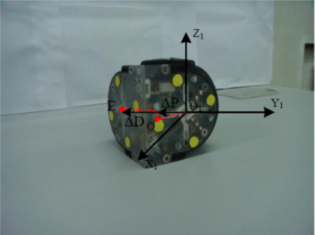
The coordinate system O₁−X₁Y₁Z₁ is attached onto the target module to demarcate its orientation, where O₁ is put on the centre of symmetry of the features, and O is the centre of field of vision (see Figure 8). The projection in the axis Y₁ of vector $\vec{O 1 O}$ , i.e., ΔP is the horizontal offset. The sign of ΔP determines the direction of movement of the vision sensor relative to the target module.

Figure 8.

Coordinate system establishment

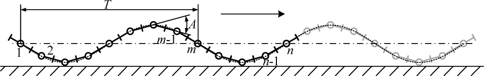
We can distinguish the docking surface as mentioned above and obtain the centre of symmetry of the circular features on the lateral surface, as indicated by the dashed line in Figure 8. The projection in the axis Y₁ of vector $\vec{O 1 E}$ is denoted ΔD, whose sign indicates the direction for the angle adjustment for the motion module.

The coordinate O₂-X₂Y₂Z₂ is attached on the sensory module to demarcate the orientation of the sensory module. For calculating the angle of adjustment, the O₂-X₂Y₂Z₂ is translated to the same origin with O₁. The features are marked as P₁, P₂, P₃, P₄ as shown in Figure 9, and the parameters L₁, L₂ are the projection of the line segments P₁P₃, P₂P₄ along Y₁, Z₁ in the projection coordinate system. The coordinate system O₂-X₂Y₂Z₂ rotates around the Z₁ axis relative to O₁-X₁Y₁Z₁ for Ψ, where cosΨ = L₁/L₂. From the relative orientation of the motion module group with respect to the target module, we can see that the necessary angular displacement φ for the module group to perform equals Ψ, as shown in Figure 9, i.e.,

Figure 9.

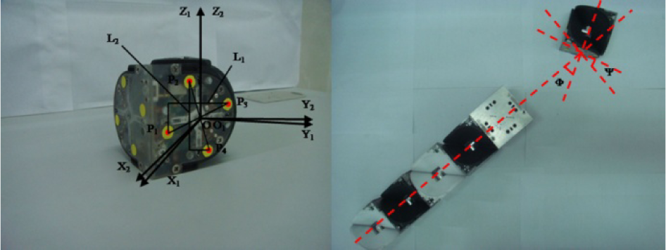
Analysis for relationship in orientation

ϕ = ψ = \arccos (L_{1} ∕ L_{2})

(6)

We set the movement rule for the pre-positioning parameter adjustment:

Rule 1 L₂ < 0.7 H& | ΔP |>| ΔP_Tol |→ if ΔP > 0, motion module group rotates to the right until | ΔP |<| ΔP_Tol | is satisfied, and vice versa;

Rule 2 L₂ < 0.7 H& | ΔP |<| ΔP_Tol |→ if ΔP > 0, motion module group moves forward as well as rotates to the right, and vice versa;

Rule 3 L₂ ⊂ (0.7 ~ 0.8)H& | Δφ |>| Δφ_Tol |→ if ΔD > 0, motion module group rotates to the left for | Δφ |<| Δφ_Tol |, and vice versa;

Rule 4 L₂ ⊂(0.7 ∼ 0.8)H& | Δφ|<| Δφ_Tol | & | ΔP |>| ΔP_Tol |→ if ΔP > 0, motion module group rotates to the left for one step, then moves backward, and rotates to the right for one step, until | ΔP |<| ΔP_Tol |, vice versa. (See Figure 10.)

Figure 10.

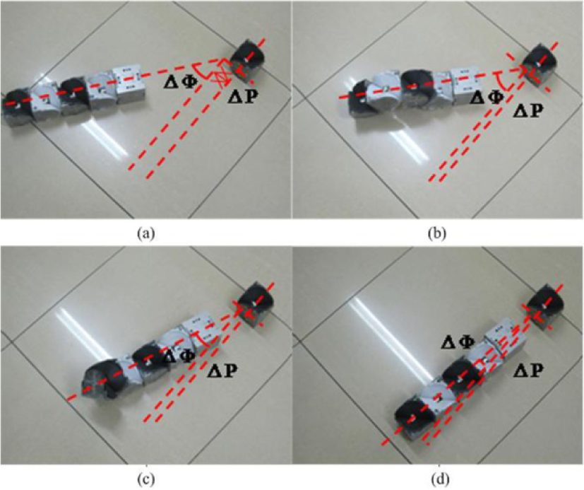
ΔP adjustment process in Rule 4. (1) The docking surface parallels to that of the target module but ΔP<0. (2) The tail of the motion group rotates to the right. (3) The tail of the motion group moves backward to eliminate the error of ΔP. (4) The tail rotates to the left again to recover the parallel state between the surface of docking and that of target module.

In the above procedures, | ΔP_Tol | is the allowable horizontal offset tolerance, | Δφ_Tol | is the allowable angular displacement tolerance, and H is the height of the view field. When the motion module is further away from the target module, i.e., L₂ < 0.7H, with Rules 1 and 2 the motion module group can approach the target module in the correct direction. When the motion module is close to the target module, i.e., L₂ ⊂ (0.7~0.8)H, Rule 3 allows the motion module group to keep the docking surface parallel to that of the target module, and the introduced horizontal error could be compensated with Rule 4. For example, when the docking surface is parallel to that of the target module but ΔP<0, as shown in Figure 9, the tail of the motion group rotates to the right and moves backward to eliminate the error of ΔP. As a sacrifice, the docking surface deviates from that of the target module, so the tail rotates to the left again to recover the parallel state.

3.2 Hall-sensor-guided precise positioning

After pre-positioning preparation, precise positioning is initialized for docking. The four Hall sensors can measure their distances to the corresponding magnets on the docking surface of the target module, and compute the parameters for the motion module group for adjustment. We set up the coordinate system O₁-X₁Y₁Z₁ and O₂-X₂Y₂Z₂ on the geometric centre of the docking surfaces of the target module and the sensory module. Based on the establishment of these coordinate systems, the kinematics analysis is described to illustrate the progress of the parameter acquisition. The following conditions must be satisfied: X₁ and X₂ are coincident and perpendicular to the docking surface; Y₁ and Y₂ are along the horizontal direction; Z₁ and Z₂ perpendicular to the horizontal surface. (See Figure 11 for illustrations.)

Figure 11.

Coordinate system for precise docking

By analysing the spatial relative position and orientation relationship, O₂-X₂Y₂Z₂ can be aligned with O₁-X₁Y₁Z₁ by first moving along X₁ for Δdx, then along Y₁ for Δdy, and finally rotating around Z₂ for Δθ_z. The relevant coordinate transformation matrix is:

\begin{array}{l} T = T_{x y} \cdot R (Z_{2} \cdot Δ θ_{z}) \\ = [\begin{matrix} 1 & 0 & 0 & Δ d x \\ 0 & 1 & 0 & Δ d y \\ 0 & 0 & 1 & 0 \\ 0 & 0 & 0 & 1 \end{matrix}] [\begin{matrix} \cos Δ θ_{z} & - \sin Δ θ_{z} & 0 & 0 \\ \sin Δ θ_{z} & \cos Δ θ_{z} & 0 & 0 \\ 0 & 0 & 1 & 0 \\ 0 & 0 & 0 & 1 \end{matrix}] \\ = [\begin{matrix} \cos Δ θ_{z} & - \sin Δ θ_{z} & 0 & Δ d x \\ \sin Δ θ_{z} & \cos Δ θ_{z} & 0 & Δ d y \\ 0 & 0 & 1 & 0 \\ 0 & 0 & 0 & 1 \end{matrix}] \end{array}

(7)

We use vector $\vec{m 1}$ to denote the pose of the magnet on the target surface in O₁-X₁Y₁Z₁, $\vec{m 2}$ for the pose of the corresponding Hall sensor on the sensory module in O₂-X₂Y₂Z₂, and $\vec{d 1}, \vec{d 2}, \vec{d 3}$ and $\vec{d 4}$ for the spatial vector for the four magnets towards the Hall linear sensors. These vectors are the input parameters from the Hall linear sensors and the target of measurement is to gain the parameters Δdx, Δdy and Δθ_z. We can derive the following relationship:

\begin{array}{l} {\vec{d}}_{1} = \vec{m_{2} m_{1}} - \vec{m_{1}} = T \cdot \vec{m_{1}} - \vec{m_{1}} \\ = [\begin{matrix} \cos Δ θ_{z} & - \sin Δ θ_{z} & 0 & Δ d x \\ \sin Δ θ_{z} & \cos Δ θ_{z} & 0 & Δ d y \\ 0 & 0 & 1 & 0 \\ 0 & 0 & 0 & 1 \end{matrix}] [\begin{matrix} 0 \\ r \sin α \\ r \cos α \\ 1 \end{matrix}] \\ = [\begin{matrix} - r \sin Δ θ_{z} \sin α + Δ d x \\ (\cos Δ θ_{z} - 1) r \cos α + Δ d y \\ 0 \\ 0 \end{matrix}] \end{array}

(8)

where r is the radio distance from the magnet to the module centre and α is to the acute angle between r and the axis of the coordinate system. Note that both r and α are known. Hence we have:

| \vec{d_{1}} |^{2} = {(- r \sin Δ θ_{z} \sin α + Δ d x)}^{2} + {[(\cos Δ θ_{z} - 1) r \cos α + Δ d y]}^{2}

(9)

| \vec{d_{2}} |^{2} = {(r \sin Δ θ_{z} \cos α + Δ d x)}^{2} + {[(1 - \cos Δ θ_{z}) r \cos α + Δ d y]}^{2}

(10)

| \vec{d_{3}} |^{2} = {(r \sin Δ θ_{z} \sin α + Δ d x)}^{2} + {[(1 - \cos Δ θ_{z}) r \cos α + Δ d y]}^{2}

(11)

| \vec{d_{4}} |^{2} = {(- r \sin Δ θ_{z} \cos α + Δ d x)}^{2} + {[(\cos Δ θ_{z} - 1) r \cos α + Δ d y]}^{2}

(12)

Similarly, we have established the relationship between the measurement values $∣ \vec{d 2} ∣, ∣ \vec{d 3} ∣$ and $∣ \vec{d 4} ∣$ and parameters Δdx, Δdy and Δθ_z. We can compute the parameter values by solving the four equations.

3.3 Summary of entire docking control

The vision sensor obtains the image information. The acquired image goes through features extraction, which yields the pre-positioning adjustment parameters Δφ and ΔP. The motion module group approaches the target, making sure that the field of vision of the sensory module is facing directly towards the centre of the docking surface on the target module via ΔP adjustment. When it is close enough to the target module, rotation adjustment for the value Δφ will ensure the two docking surfaces are parallel to each other. However, the rotation of the module group could result in ΔP's going beyond the allowable range, in which case we adjust Δφ using Rule 4. The vision sensor is turned off until the motion module group is adjusted to satisfy Δφ < 3°& ΔP < 4 mm. After visual pre-positioning preparation, the motion module group moves forward and obtains the range information through linear Hall sensors. The docking algorithm computes Δdx, Δdy and Δθ_z. The motion module adjusts the relative position and orientation. When the conditions Δdx<1mm, Δdy<1mm, Δθ_z<2° are satisfied, the motion module group moves forward slightly, and the active module actuates the hook-type connecting mechanism to complete docking. The whole control flowchart is shown in Figure 12, where the visual pre-positioning preparation is on the left, and the precise docking adjustment process is on the right.

Figure 12.

Entire docking control flowchart

4. Experimental verification

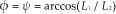
During the process of docking, the module group adjusts its relative position and orientation eventually, while the form of adjustment includes different motion patterns. For example, the sine wave motion is applied for adjusting long distances in the pre-positioning. In this motion situation, the group of motion modules is similar to the shape of the sine wave as shown in Figure 13.

Figure 13.

The motion state of the module group

It exists a certain phase difference φ between adjacent modules. The phase difference φ depends on the size of modules planned in one periodic wave. Assuming that the number of modules is m in one periodic wave, then the phase difference φ could be:

ϕ = 2 π ∕ (m - 1)

(13)

During the process of motion, the latter module repeats the previous adjacent module joint angle, by which the sine wave proceeds along the running direction. As outlined above, the relationship between the joint angle Ai of the module I and the time t can be given as:

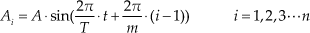
A_{i} = A \cdot \sin (\frac{2 π}{T} \cdot t + \frac{2 π}{m} \cdot (i - 1)) \begin{matrix} i = 1, 2, 3 \dots n \end{matrix}

(14)

where symbol A is the amplitude of joint angle, T donates the signal period of joint angle and n is the number of modules in the configuration. The group of motion modules consists of four modules, so we set n=m=4.

Apart from sine wave motion, the angle adjustment could also be achieved by lateral rotation at the tail module, and longitudinal rotation at the tail module produces slight forward movement to achieve a small adjustment of distance. The docking method mentioned above is applied for docking experiments with worm-shaped configuration and T-shaped configuration. These experiments will be introduced in the next sub-section.

4.1 Docking in worm-shaped configuration

The worm-shaped configuration is the simplest configuration for UBot SRR system. Docking in the worm-shaped configuration can verify the validity of the docking approach. A group of experiments is conducted in the followed situation: in the level floor, there is approximately 300 mm distance between sensory module and target module, and the module group remains at 30 degrees relative to the target module. In this initial situation, the docking process is achieved successfully and the whole pre-positioning and precise positioning take about 21 s and 26 s, respectively. The visual pre-positioning preparation is shown in Figure 14. After pre-positioning preparation, the linear Hall sensors are initialized to capture range information, and the motion adjustment parameters are calculated through the precise docking algorithm. When the adjustment is within the allowable tolerance, the motion module group moves forward slightly, and the active module actuates the hook-type connector to realize the docking process, as shown in Figure 15.

Figure 14.

Rough positioning process

Figure 15.

Precise positioning process

4.2 Docking in T-shaped configuration

The environment may be complex and dynamic for UBot SRR system, which calls for configurable versatility. For this, we experimented with two identical motion module groups to dock with a static motion module group, with the target module set as the head. The purpose is to transform to a T-shape. The results are shown in Figure 16. The required docking distance is about 100 mm from sensory module to target and the whole docking process takes 40 s. These experiments showed that our docking algorithm is very effective.

Figure 16.

Docking for T-shaped configuration

5. Conclusion

We have proposed a novel autonomous docking approach for UBot SRR without using mechanical guidance between docking surfaces by combining a hook-type connecting mechanism with multi-sensory alignment guidance. From the preliminary experimental results, some conclusions can be given, as follows:

By combining the information of visual and Hall sensors, the hunter robots accomplish the whole process of capturing, closing, aligning and connecting within the distance range of 1 metre.

The array of Hall sensors along with magnets is a simple and non-contact means by which to detect the orientation misalignments between two adjacent surfaces, and is sufficient for fine poisoning without the help of mechanical guidance.

For future work, we will add a computing unit to the sensory module, by which the image processing could be carried out in the sensory module. This revision could construct a distributed system of SRR and reduce the excessive dependence on the PC. In addition, we will simplify the rough positioning of the current algorithm, which is relatively complex and time-consuming, in order to promote the docking efficiency and shorten the time of image processing.

Footnotes

6. Acknowledgement

This work was supported by National Natural Science Foundation of China (61273316) and Self-Planned Task (NO. SKLRS201201A02) of State Key Laboratory of Robotics and System (HIT). The authors express gratitude for the financial support.

References

Fukuda

Nakagawa

(1987) A Dynamically Reconfigurable Robotic System (Concept of a System and Optimal Configurations). Robotics and IECON '87 Conferences, International Society for Optics and Photonics, pp. 588–595.

Bonardi

Moeckel

Sproewitz

. (2012) Locomotion through Reconfiguration Based on Motor Primitives for Roombots Self-Reconfigurable Modular Robots. Robotics; Proceedings of ROBOTIK 2012; 7th German Conference, pp. 1–6.

Spröwitz

Moeckel

Vespignani

. (2013) Roombots: A Hardware Perspective on 3D Self-Reconfiguration and Locomotion with a Homogeneous Modular Robot. Robotics and Autonomous Systems, 62(7), pp. 1016–1033.

Sproewitz

Laprade

Bonardi

. (2010) Roombots - Towards Decentralized Reconfiguration with Self-Reconfiguring Modular Robotic Metamodules. Intelligent Robots and Systems (IROS), IEEE/RSJ International Conference, pp. pp. 1126–1132.

Luo

Chi

. (2011) Motion Error Analysis of Modular Self-Reconfigurable Robot M-Cubes based Screw Theory. Electronic and Mechanical Engineering and Information Technology (EMEIT), 2011 International Conference, 2, pp. 859–866.

Yoshida

Murata

Kamimura

. (2003) Self-Reconfigurable Modular Robots-Hardware and Software Development in AIST. Robotics, Intelligent Systems and Signal Processing, Proceedings of IEEE International Conference, 1, pp. 339–346.

Kurokawa

Tomita

Kamimura

Kokaji

Hasuo

Murata

(2007) Self-Reconfigurable Modular Robot M-TRAN: Distributed Control and Communication. Proceedings of the 1st International Conference on Robot Communication and Coordination, pp. 21.

Kurokawa

Tomita

Kamimura

. (2008) Distributed Self-Reconfiguration of M-TRAN III Modular Robotic System. The International Journal of Robotics Research, 27 (3–4), pp. 373–386.

Kurokawa

Yoshida

Tomita

. (2006) Self-Reconfigurable M-TRAN Structures and Walker Generation. Robotics and Autonomous Systems, 54(2), pp. 142–149.

10.

Murata

Kurokawa

(2007) Self-Reconfigurable Robots. Robotics & Automation Magazine, 14(1), pp. 71–78.

11.

Hossain

S G M

Nelson

C A

Dasgupta

(2012) Hardware Design and Testing of ModRED: A Modular Self-Reconfigurable Robot System. Advances in Reconfigurable Mechanisms and Robots I, pp. 515–523.

12.

Han

Ranasinghe

Barrios

. (2012) An Online Gait Adaptation with Superbot in Sloped Terrains. Robotics and Biomimetics (ROBIO), 2012 IEEE International Conference, pp. 1256–1261.

13.

Hou

Shen

W M

(2010) On the Complexity of Optimal Reconfiguration Planning for Modular Reconfigurable Robots. Robotics and Automation (ICRA), 2010 IEEE International Conference, pp. 2791–2796.

14.

Shen

W M

Krivokon

Chiu

Everist

Rubenstein

Venkatesh

(2006) Multimode Locomotion via SuperBot Reconfigurable Robots. Autonomous Robots, 20(2), pp. 165–177.

15.

Maye

(2007) Control of Locomotion in Modular Robotics, Biologically Inspired Robotics Group [Master's thesis]. École Polytechnique Fédérale de Lausanne (EPFL).

16.

Möckel

Jaquier

Drapel

Dittrich

Upegui

Ijspeert

(2006) YaMoR and Bluemove - An Autonomous Modular Robot with Bluetooth Interface for Exploring Adaptive Locomotion. Climbing and Walking Robots, Springer Berlin Heidelberg, pp. 685–692.

17.

Moeckel

Jaquier

Drapel

Dittrich

Upegui

Ijspeert

A J

(2006) Exploring Adaptive Locomotion with YaMoR, A Novel Autonomous Modular Robot with Bluetooth Interface. Industrial Robot: An International Journal, 33(4), pp. 285–290.

18.

Roufas

Zhang

Duff

Yim

(2001) Six Degree of Freedom Sensing for Docking using IR LED Emitters and Receivers. Experimental Robotics VII, Springer Berlin Heidelberg, pp. 91–100.

19.

Shen

W M

Will

(2001) Docking in Self-Reconfigurable Robots. Intelligent Robots and Systems, Proceedings of IEEE/RSJ International Conference, 2, pp. 1049–1054.

20.

Wei

Cai

Wang

(2010) Sambot: A Self-Assembly Modular Robot for Swarm Robot. Robotics and Automation (ICRA), IEEE International Conference, pp. 66–71.

21.

Liu

Zheng

Wei

(2011) Monocular Camera Based Guiding and Positioning Strategy for Docking of a Distributed Swarm Flight Robot. Robotics and Biomimetics (ROBIO), IEEE International Conference, pp. 325–330.

22.

Murata

Kakomura

Kurokawa

(2006) Docking Experiments of a Modular Robot by Visual Feedback. Intelligent Robots and Systems, IEEE/RSJ International Conference, pp. 625–630.

23.

Metta

Gasteratos

Sandini

(2004) Learning to Track Colored Objects with Log-Polar Vision. Mechatronics, 14(9), 989–1006.

24.

Zhu

Zhao

Cui

. (2013) Design and Implementation of UBot: A Modular Self-Reconfigurable Robot. Mechatronics and Automation (ICMA), 2013 IEEE International Conference, pp. 1217–1222.

25.

Zhao

Cui

Zhu

Tang

(2012) UBot: A New Reconfigurable Modular Robotic System With Multimode Locomotion Ability. Industrial Robot, 2012, Vol. 39 Iss. 2, pp. 178–190.

A Multi-Sensory Autonomous Docking Approach for a Self-Reconfigurable Robot without Mechanical Guidance

Abstract

Keywords

1. Introduction

2. Physical platform of UBot

2.1 Basic module

2.2 Sensory module

3. Docking in self-reconfigurable robot

3.1 Visual-sensor-guided rough positioning

3.1.1 Feature extraction

3.1.2 Analysis for extracted feature

3.2 Hall-sensor-guided precise positioning

3.3 Summary of entire docking control

4. Experimental verification

4.1 Docking in worm-shaped configuration

4.2 Docking in T-shaped configuration

5. Conclusion

Footnotes

6. Acknowledgement

References