Sage Journals: Discover world-class research

Abstract

Parallel robots are specially designed to perform high-precision tasks. Nevertheless, manufacturing, assembling and control issues can reduce their capacity to perform adequately. Observing the acquired measurement data with high-precision devices - such as laser-based instruments - it is not surprising that the error data follows patterns or have a structure because, in many cases, the greatest error comes from a mechanical bias introduced by manufacturing issues. Even though we cannot determine with certainty where the error comes from, a pattern in the measured data suggests that it is feasible that it can be modelled and corrected - in a significant proportion - by purely software applications, without the need of disassembling or re-manufacturing any component. This work deals with the problem of finding a mathematical model which adequately fits the error data from the legs of a general Gough-Stewart platform. Hence, we obtain an expression which can be subtracted from the control parameters in order to compensate the inherent mechanical error in the legs. The purpose of this article is two-fold: 1) to present numerical results of the beneficial effects of the error compensation in the legs as well as in the end-effector, and 2) to introduce a numerical methodology to find a model for error compensation and to numerically simulate its effects. Numerical, graphical and statistical evidence of the error improvements, according this methodology, is provided.

Keywords

Parallel Robots Modelling Error Simulation Compensation

1. Introduction

Parallel robots have become an excellent solution for applications where precise positioning and orientation are needed. Although their workspace is limited as compared to serial robots, parallel robots take advantage of their dynamic stability, high stiffness and high pose accuracy. Therefore, they are suited to very precise applications, such as machine tools, surgery devices and scientific instruments, like radio-astronomy telescopes. Due to their design, there is no one-to-one relationship between controllable variables and degrees-of-freedom (DOF), and each controllable variable affects all DOFs (and vice versa). Therefore, the determination of an end-effector pose requires special algorithms. Besides the complexity of the mechanism's kinematics, the pose error depends mainly on the accuracy of the actuators, the control scheme and the elastic deformations.

One application where high accuracy is needed is in machine tools. In this area, a large number of strategies for error modelling and compensation have been studied and can be considered as consolidated [1], [2]. There are a lot of works dealing with the accuracy of serial manipulators and conventional machine tools. Error modelling, studies of manufacturing and assembly errors on pose accuracy and different calibration approaches are examples of topics in these areas. In contrast, in order that a parallel robot can be applied as a machine tool, calibration strategies should be clearly defined [3]. Conventional machine tools consist on three mutually orthogonal axes and two perpendicular rotating axes. Each DOF moves independently, and each is controlled by a separate driver. Thus, the kinematics and dynamics models are simpler than in a parallel robot. For parallel robots, the pose and twist of the end-effector depend on the simultaneous movement of every driver, and the kinematic function that relates each of the individual joints contributes to the accuracy of the moving platform. The global error of the end-effector is the main concern. This error could be a function of many error sources, and there is no unique method for estimating the actual pose. The most significant error sources can be classified as manufacturing errors, joint run-out, ball screw deviations, transmission errors, elastic and thermal deformations, sensor accuracy, and algorithm and truncation errors. Manufacturing errors are caused by geometrical deviations of machined parts and assembly errors. Joint run-outs are a combination of a joint's gaps and assembly errors and the joint movement. Elastic deformations are produced by external and gravitational loads applied to the links. Thus, they are a function of the posture of the mechanism. They can be compensated only if the elastic deformation of the robot can be characterized [4]. Pose and twist sensors usually have a defined accuracy and, in many cases, the error are small enough so that their contribution to the pose error is minimal. However, for very accurate mechanisms, their contribution is significant and must be taken into consideration. Incidentally, the kinematic model is one of the main elements of the control algorithm. It contributes to the pose accuracy with truncation errors in the kinematic model, control loop and time response.

Usually, error compensation methods can be divided into two areas: 1) hardware and mechanical methods, and 2) Software methods. The first class of approaches uses compensation error procedures through some mechanical means. Software approaches to compensating errors become useful when it is difficult to implement the hardware or mechanical methods. Their main advantage is that they can be implemented without the need for the disassembly or re-manufacture of any component of the robotic system.

As for so-called ‘parallel kinematic machines’ (PKMs), in [5] it is attributed the source of errors to the uncertainties of the theoretical model, such as the coordinates of the base and moving platform joint centres, as well as the link lengths in the initial position. In [6] it was reported the measurement and analysis of geometrical errors through a kinematic model and experimental measurements using conventional metrology tools. He used variation analysis of the kinematic model to describe how errors in the real geometry of the machine components generate parametric errors in the moving platform. In [7] it was emphasized that the kinematic and dynamic behaviour of a parallel mechanism is strongly influenced by joint geometrical errors due to manufacturing tolerances and assembly errors. In [8] it was reported that the spherical joints’ distance located at the leg end - which is the leg length - is fundamental for platform accuracy positioning. This condition is critical in the actual position of the moving platform, and it was also found in the present work. In [9] it was established kinematic modelling and error modelling using the Jacobian matrix method for a TAU robot. In [10] it is described an error compensation method for parallel mechanisms. He identified two types of errors, namely those related to elastic and thermal deformations, and those related to manufacturing deviations and backlash. In [11] it is presented a geometric approach for the computation of local maximum position and orientation errors. They used actuator inaccuracies as input errors. In [12] it is proposed a method for estimating the accuracy of three-DOF planar parallel robots. In [13] it was predicted the pose errors that are caused by joint clearances. In [14] it was proposed a new calibration method. Their method allows for the identification of joint offsets through the evaluation of the leg's parallelism with respect to the ground reference plane. In [15] it was developed a calibration algorithm based on constraining two of the orientation angles. They measured the orientation of the moving platform with two precise inclinometers (biaxial inclinometer) and through the kinematic model they found the actual overall position. These kinds of measurement devices are less frequently used, and while they are more accurate, they are also more expensive. More recently, an approach for modelling quasi-static errors in a five-axis Gantry machine tool was presented in [16]. Quasi-static error is a common classification for geometric, kinematic and external load-induced errors. In sum, the task of characterizing and modelling errors and using them in a software compensation system can be considered to be a transcendental step in enhancing the accuracy of parallel robots.

This paper presents a methodology to compensate for the leg errors of general Gough-Stewart platforms. It includes a mathematical error model which adequately fits the measurement of the displacement errors for the six legs of a parallel platform. It is well known that the effectiveness of error compensation approaches relies heavily on the error model. With this model, the modelled compensation function can be considered in a control scheme in order to compensate the inherent mechanical and displacement errors in the legs. Numerical results of the beneficial effects of the error compensation in the legs as well as in the end-effector pose are reported.

The rest of this paper is structured as follows: the second section is concerned with the Gough-Stewart platform and its problems; the third section describes the measured displacement errors, the process and the instruments employed to obtain them; the fourth section explains the proposed modelling error technique; the fifth section describes the process suggested to compensate the measurement differences; and finally, the last section provides the conclusions of this paper.

2. The Gough-Stewart platform and its kinematics

With the aim of describing useful applications of parallel mechanisms, the secondary mirror positioner of modern millimetre radio-telescopes can be employed as an illustrative example. These radio-telescopes have a large parabolic mirror (from 30 m to 100 m) that concentrates radiation into a secondary mirror. The secondary mirror must keep the focus length within a tolerance of less than 10 μm, and an orientation tolerance of less than 1 arc-sec. Since a positioner mechanism is intended as a highly precise scientific instrument, the Gough-Stewart platform architecture can be selected as being suitable (see Figure 1). Its kinematic configuration consists of a fixed plate connected by six driving legs to a moving platform.

Figure 1.

General Gough-Stewart-based parallel platform: a) actual platform, b) a scheme of the platform

Each leg has an actuated prismatic joint, a spherical joint at the fixed end, and a universal joint at the moving end. The fixed and mobile platforms have the same dimensions. In order to improve the mechanism's stability, the spherical and universal joints were located as close as possible such that they form triangular structures, as shown in Figure 1. Each actuator consists of a servo motor connected to an almost zero-backlash gearbox, and the piston rod is moved through a zero-backlash ball screw, as shown in Figure 2. The ball screw is mounted on high-precision rolling bearings.

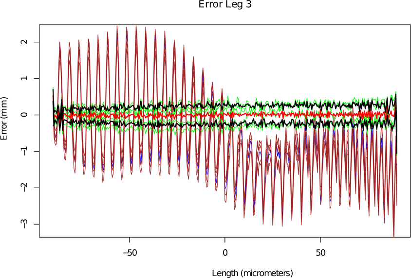
In Equation 1, E = [x, y, z, α, β, γ] represents the position and the orientation parameters of the mobile platform in the moving frame. When E is given, the problem of computing the length of each leg, L = [L₁,…, L₆], is known as the inverse kinematic problem, as denoted by the next equation:

L = F (E)

(1)

Where F represents the inverse kinematic function of the general Stewart platform. Notice that the position E is a function of the location of the mobile platform's joints, P_j, and the location of the fixed platform joints, B_j, for (j = 1,…, 6). In consequence, the inverse kinematic problem for the Stewart platform can be easily solved. On the other hand, the direct kinematics problem of the general Stewart platform cannot be algebraically solved. In this work, we employ a method to numerically solve this problem.

Figure 2.

A leg for a Gough-Stewart platform: a) actual leg, b) a CAD model and main parts

3. Measurement of the displacement errors and modelling

The desired accuracy of the control system is achieved by having a redundant encoder measurement. The main encoder is a linear encoder that measures the actual leg displacement. For each leg, the difference between the commanded leg length and the actual length has been measured. The difference was measured with a laser interferometer with 0.1 μm nominal accuracy, [17]. The calibration equipment is shown in Figure 3. It consists of a leg, a laser and an interferometer.

The ball screw is the element with the largest displacement error; it has a linear deviation of 9 μm/m.

Figure 3.

Data acquisition with calibration equipment RENISHAW ML10

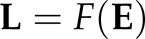
For each leg, six sets of 361 measurement differences were obtained. The length of each leg is variable depending on a ball screw actuator, thus, in order to take the measurements, they are positioned for having the half of the maximum length. Hence, these displacements are relative to this position. A set of these measured errors is presented in Figure 4. As can be observed, they seem quite similar, with small changes in the scale and the y position (error axis). The lengths of the legs are controlled by using the ball screw actuator as mentioned before; as a result, it is logical that a mechanism which has been similarly manufactured should also share the same mechanical bias. Fortunately, the error presents a pattern - by graphical analysis, one can observe that the errors can be seen as a sum of periodic functions. Hence, the purpose of this section is to find a explicit mathematical function which represents the displacement error and can be used to compensate for it.

Figure 4.

A set of displacement error measures of the six legs for the Gough-Stewart platform. The units are micrometres.

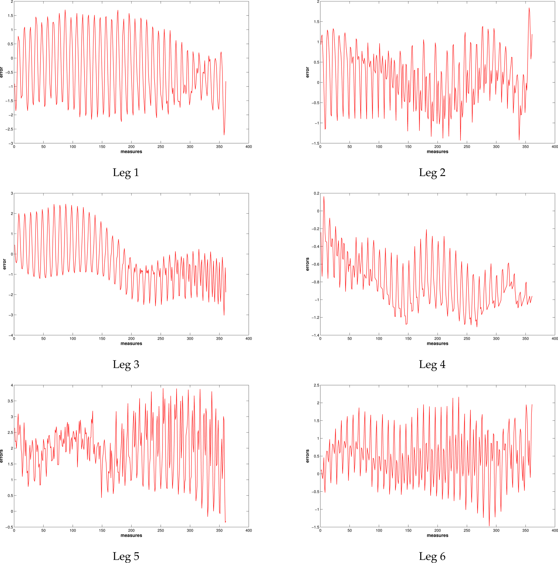
The Fourier transform constitutes a well-known approach to obtaining the frequency components from a given signal. In our case, given the characteristics of the measured displacement errors, the discrete Fourier transform (DFT) is used (see Equation 2). The DFT transforms a defined function into a finite discrete interval of the frequency domain representation. By using Equation 2, a set of N complex numbers is transformed into another set of N numbers. Only the first half of the vector delivered by Equation 2 is useful, considering that the second half is only a reflection of the first:

F_{k} = \sum_{n = 0}^{N - 1} f_{n} \cdot e^{- i 2 π \frac{k}{N} n}

(2)

In Equation 2, F_k represent the amplitude and phase of the different sinusoidal components of the input function. The amplitude of each component in the frequency domain is computed according Equation 3, the phase is computed according to Equation 4, and finally, the matched frequency is obtained with Equation 5:

Figure 5.

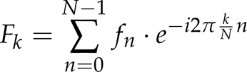
Compensation for displacement leg errors of the Gough-Stewart platform: brown lines - set of measured data for each leg; blue line - error compensation function; red line - mean of compensated displacement errors; green lines - compensated errors for each set of measures; black lines - plus and minus of the standard deviation for the compensated displacement errors. N.B. The units are micrometres.

Figure 6.

Original displacement error of Leg 3, the compensation function and the compensated error

A_{k} = | F_{k} | = \sqrt{R e {(F_{k})}^{2} + I m {(F_{k})}^{2}},

(3)

ϕ_{k} = \arg (F_{k}) = \arctan (I m (F_{k}), R e (F_{k})),

(4)

w_{k} = k, f o r k = 0.. N - 1.

(5)

Once the Fourier transform is obtained, the original data can be sampled from Equation 6, which uses the attained parameters:

f (t) = \sum_{k = 1}^{N} A_{k} \cos (2 π ω_{k} t + ϕ_{k}) .

(6)

Figure 7.

Histogram of the leg errors of the Gough-Stewart platform, Legs 1–3. Left: original displacement error. Right: compensated error.

In order to use Equations 2, 3, 4 and 6 in our context, it should be noted that: the signal {x_n, f_n} is the displacement error data, x_n is the length of a given leg and f_n is the corresponding error at that position. As can be observed, function 6, which is used to rebuild the error function, does not depend on the leg's length x_n directly. Therefore, a transformation must be applied following Equation 7. It needs the position of the half of the leg (which is the same as used for measurement differences), but in its nominal value:

t = 2 (x - 1095.84992501338 + 90) / N .

(7)

Once frequencies, phases and amplitudes are found, the most important among them are selected in order to reduce the model complexity. This is achieved by reducing the number of involved parameters - in this case, we use the most important 100 parameters of amplitudes, frequencies and phases. The resulting model of the sums of the cosines can then be used to correct or compensate the displacement error in the legs. The complete methodology to compute the model using the Fourier transform is presented in Algorithm 1. It is executed for each leg. The input is a pair of vectors x and f. x are the displacements of a given leg and f is the corresponding error for that leg. In Step 1, we compute the mean of the error; in Step 2, the mean is used to translate the error to zero. It is to see that this step removes the average bias of the leg. In Step 3, the Fourier transform is computed and stored in F. Using the Fourier transform, we compute the amplitudes in Step 4, the phases in Step 5, and the corresponding frequencies w in Step 6. The greatest amplitudes are those which contribute the most to representing the error. The algorithm returns the amplitudes with the highest contribution as well as the phases, frequencies and the average error (this information is actually a mathematical model of the measured error). If the measured error is always the same, this model is a perfect representation and can be used to compensate the error perfectly. Hence, the difference between the model and the real error results because each time it is measured, the measurement is different (but similar). The more that similar each measurement is to every other, the more efficient the proposed methodology will be.

Figure 8.

Histogram of the leg errors of the Gough-Stewart platform, Legs 4–6. Left: original displacement error. Right: compensated error.

Figure 9.

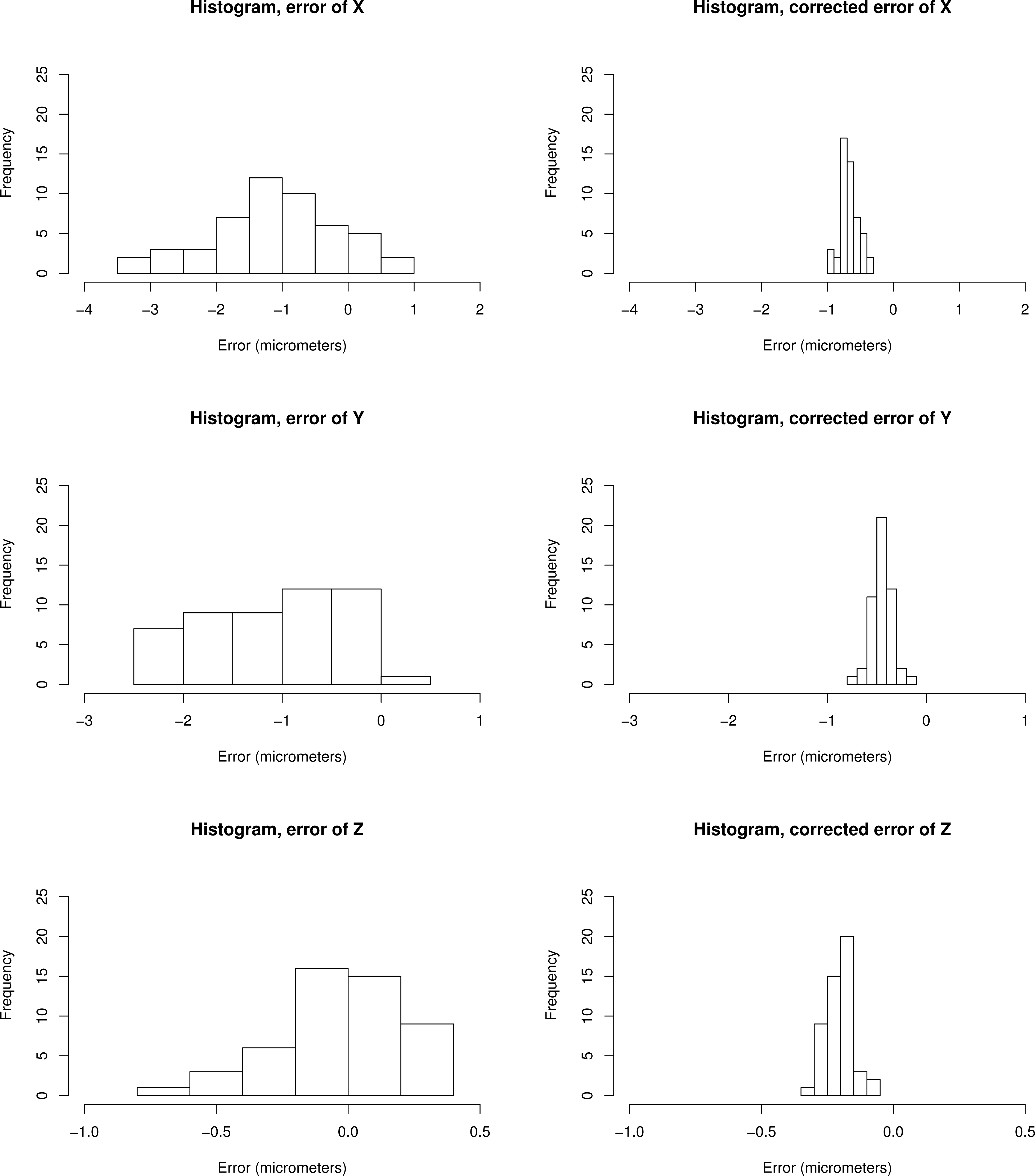
Histogram of the end-effector position errors for the Gough-Stewart platform. Left: original error. Right: compensated error.

Additionally, graphical evidence of the procedure's results are shown in Figure 5. For each leg, the graphs correspond to six sets of measured displacement errors, the error modelling function and the statistical treatment of the compensated displacement errors. From Leg 4 in Figure 5, we can note that when the displacement errors exhibit random behaviour, it is difficult to compensate for them. In contrast, when the displacement errors present a defined pattern, it is easier to compensate for them, as can be seen for Legs 2, 3 and 5 in Figure 5. A possible explanation of such deterministic patterns is the physical error introduced by the leg screw; hence, it is quite possible to find this kind of deterministic pattern in the errors, and in consequence it is an adequate assumption that this error can be compensated for by a deterministic periodic function, such as the Fourier transform proposed in this work. The relevance of obtaining such an error compensation function is that it can be used in a control scheme.

Figure 10.

Histogram of the end-effector orientation errors for the Gough-Stewart platform. Left: original error. Right: compensated error.

Input: A pair of vectors x and f, {x_n, f_n} for n = 1..N. Where x are the displacements of a single leg and f is the associated error. For each position, x_n corresponds to an error value f_n. The algorithm is executed once for each leg of the parallel robot. /* Centering the data around 0. */ 1. f_mean ← mean(f); 2. f ← f – f_mean; /* Compute the Fourier transform. */ 3. F ← fft(f); /* Compute the amplitudes. */ 4. A ← Mod(F[1: (N/2)]); /* Compute the phases. */ 5. ϕ ← Arg(F[1: (N/2)]); /* Compute the frequencies. */ 6. ω ← (0: (N/2 – 1)) /* Select the indexes of the greatest amplitudes. */ 7. ix ← sort(A, increasing, return.index); /* Returns the M data with the greatest amplitudes and the mean of the original function. */ return A[ix[1: M]],ϕ [ix[1: M]],ω[ix[1: M]],f_mean

Algorithm 1: Parameter computation for modelling the displacement leg errors as a sum of cosines

Table 1.

Range and absolute value of the errors for the original data and for the compensated error. *|Error| = Error absolute value. N.B. The units are micrometres.

Measure	Leg1	Leg 2	Leg 3	Leg 4	Leg 5	Leg 6
Maximum original error	9.7000	9.7000	9.7000	9.7000	9.7000	9.7000
Minimum original error	–19.6000	–19.6000	–19.6000	–19.6000	–19.6000	–19.6000
Maximum compensated error	3.2109	2.3854	3.1037	4.6861	3.4409	2.6793
Minimum compensated error	–4.0669	–2.4778	–3.8256	–2.7489	–2.2658	–3.2292
Percentage of reduction of the error range	76.60%	83.11%	77.36%	72.46%	82.22%	79.83%
Average of original \|Error\|*	3.8981	3.9629	3.9244	3.9454	3.8934	3.9283
Average of compensated \|Error\|*	0.4320	0.4120	0.4252	0.5011	0.6235	0.5106
Percentage of reduction of the \|Error\|* average	88.92%	89.60%	89.17%	87.30%	83.99%	87.00%

The Figure 6 shows the original displacement error, the compensation function and the resulting error when subtracting the compensation function defined in Equation 6 from the original error. Notice that the error compensation function and the measured error are quite similar. The following section completes the procedure for the error compensation for the end-effector.

4. Error compensation in the legs and the end-effector pose

Using the methodology just described, we compute the compensation function according to Equation 6. The results of compensating for the displacement leg errors are described in Table 1.

In order to show the advantages of the methodology just presented in this article, we perform the following experiments:

Generate random configurations of the end-effector by using the inverse kinematics and finding the corresponding leg lengths.

If the leg lengths are within the range of the measures, then we use the error data and linear interpolation to sum the corresponding error for each leg.

Solve the direct kinematics for the new lengths in order to determine the end-effector coordinates and angles, and store the values for the comparison presented below.

Use the compensation function in Equation 6 to compensate for the displacement error, solve the inverse kinematics with the compensated lengths, and store the values for the comparison presented below.

Following the steps given above, we can analyse the resulting error in the legs by observing the histograms presented in Figure 7 and 8. The left side shows the frequencies of the errors before compensation, and the right side after compensation. As can be seen, very similar compensation is achieved in the legs as achieved in the end-effector.

The range of the error is somewhat lower in the compensated error than in the original.

The compensated error is closer to 0 than the original.

The compensated highest frequencies in the compensated histogram error are higher than the highest frequencies in the original error histogram. This is important if we consider that the compensated error has the highest frequencies around 0. Hence, most of the measures are adequately compensated for.

As can be observed, the methodology just presented not only diminishes the error but in addition it changes the pattern. We can infer this behaviour by looking at Figure 6, where we can observe that the original error data has a pattern and the resulting compensated function seems to be a kind of random function.

Finally, we can analyse how the displacement leg errors and their corrections affect each of the parameters of the configuration in the end-effector. The improvement in position, according to our experiments, is reported in Table 2. Notice that these measures can represent a sample of the workspace. In this vein, it must be remarked upon that not all of the randomly generated points can be solved with the desired precision, as it is very possible that many points cannot be physically realized. We consider that the direct kinematics are successfully solved if we get an error norm that is less than 1 × 10⁻⁴ using the solver presented in [18].

We tackle the direct kinematics problem for general Gough-Stewart platforms using a hybrid optimizer. This is based on probabilistic learning (estimation of distribution algorithms) by taking advantage of the adequate generation of starting points for the Dogleg method, without a priori knowledge.

Notice that the error norm guarantees that the numerical error for each leg is less than or equal to 1 × 10⁻⁴; thus, we avoid numerical error biases for the results. Nevertheless, the results could be biased by the random points used, due to the configurations that can be used to physically constrain the possible positions of the legs. As can be seen in Table 2, the range of the error is nonetheless reduced significantly and the error average is reduced as well. The explanation for this is the bias that we considered above. Hence, by considering specific paths or work areas, we can find the bias in the positions of the end-effector and compute a more precise compensation. In addition, notice that the histograms of the end-effector positions in Figure 7 and 8 can be centred around zero by simply applying an arithmetic difference to the compensation. As mentioned, in this case the histogram is not exactly around zero because only certain positions can be physically achieved. If we had known a priori which these points were (for example, if we had known an a priori path of the end-effector), then a more precise model could have been computed. Hence, in practice, if we know a priori the path or work area of the end-effector, more precise compensation can be calculated for such a path within the same range of error but actually centred around zero. The same behaviour can be observed in Figure 10, where Angle 3 is zero because it has no practical usage in radio-telescope applications.

Table 2.
Measures of the accuracy improvement in the end-effector pose: x,y, z in micrometres, and Angle 1 and Angle 2 in radians.

Measure x y z Angle 1 Angle 2

Maximum original error 0.8783 0.1403 0.3828 3.557e-3 2.88e-3

Minimum original error –3.496 –2.318 –0.6538 3.337e-4 –6.362e-4

Maximum compensated error –0.3371 –0.1758 –0.07755 1.5e-3 1.14e-3

Minimum compensated error –0.9698 –0.7050 –0.3047 9.687e-4 8.286e-4

Percentage of range error reduction 85.54% 78.47% 78.08% 83.54% 91.043%

Average of original |Error|^* 1.202 1.109 0.1886 1.965e-3 1.116e-3

Average of compensated |Error|^* 0.6639 0.4520 0.2044 1.274e-3 9.692e-3

Measure	x	y	z	Angle 1	Angle 2
Maximum original error	0.8783	0.1403	0.3828	3.557e-3	2.88e-3
Minimum original error	–3.496	–2.318	–0.6538	3.337e-4	–6.362e-4
Maximum compensated error	–0.3371	–0.1758	–0.07755	1.5e-3	1.14e-3
Minimum compensated error	–0.9698	–0.7050	–0.3047	9.687e-4	8.286e-4
Percentage of range error reduction	85.54%	78.47%	78.08%	83.54%	91.043%
Average of original \|Error\|^*	1.202	1.109	0.1886	1.965e-3	1.116e-3
Average of compensated \|Error\|^*	0.6639	0.4520	0.2044	1.274e-3	9.692e-3

It is worth noting that the error range in the end-effector pose is reduced to the same scale as the reduction that we performed in the legs.

5. Conclusions

This work presents a methodology to compensate the displacement leg errors of general Gough-Stewart platforms. The methodology can be applied to any parallel mechanism taking into account the following considerations:

The error data must present a pattern. This methodology is intended for deterministic errors which follow a pattern, as can be seen in Figure 4; the error does not seem to be generated from underlying stochastic phenomena but rather from a deterministic issue. Moreover, the errors are quite similar for the six legs; hence, the hypothesis that the bias is due to a mechanical, manufacturing or assembly issue is quite plausible. These reasons are important because: 1) If the error comes from stochastic phenomena, it must therefore be modelled as a random variable with some underlying distribution, and the compensation effectiveness must be tested according to statistical evidence. 2) If the error comes from deterministic phenomena (or else in a greatest proportion), then our a deterministic function must be represented accurately, not only according to the data we get from physical experiments, but also within the whole continuous range of application. Thus, the interpolation used in this work makes sense. These two assumptions have been adopted in this work based on the analysis of the empirical evidence plotted and discussed throughout the paper.

The direct and inverse kinematics must be solved with sufficient accuracy (an least an order of magnitude lower than the physical error) in order to avoid an erroneous interpretation of the numerical results.

The number of parameters must be chosen according to the desired error reduction and the simplicity of the model. Notice that there is a compromise between the number of parameters and the error compensation. If the error data present only low frequencies, few parameters are needed.

According to our results, the range of each leg's error is reduced by between 80 and 90 %. A similar reduction is achieved in the end-effector. The numerical, graphical and statistical measures and plots show that the proposal reduces the error considerably.

Finally, in the future we will contemplate using different functions which are not directly derived from the Fourier transform. Notice that the Fourier transform imposes the frequencies used for representing the function, and as such perhaps a simpler model could be used if the basis functions were different to those used in the Fourier transform.

In addition, the methodology could be applied to other mechanisms, wherever it is possible to obtain measured differences between nominal and actual values of the link/joint parameters. Finally, a stochastic version of the method must be proposed.

Footnotes

6.

Eusebio Hernandez would like to thank SIP IPN for its financial support, under projects SIP 20121377 and 20144318. The authors are also grateful to CONACYT-Mexico for supporting part of this project through grant CB-2011-01-169132.

References

Kiridena

V.S.B.

and Ferreira

P.M.

. Computational approaches to compensating quasistatic errors of three-axis machining centers. International Journal of Machine Tools and Manufacture, 34(1): 127–145, 1994.

Kiridena

V.S.B.

and Ferreira

P.M.

. Kinematic modeling of quasistatic errors of three-axis machining centers. International Journal of Machine Tools and Manufacture, 34(1): 85–100, 1994.

Jean Pierre Merlet. Parallel robots: Open problems. In ASME Conference DECT, 2002.

Angeles

Jorge

. On the nature of the cartesian stiffness matrix. Ingenieria Mecanica Tecnologia y Desarrollo, 3(5): 163–170, 2000.

Ziegert

J. C.

. Volumetric performance of hexapod machine tools. Technical Report Internal Report 13, Hexapod Machine Tool Users Group, 1996.

Soons

J. A.

Error analysis of a hexapod machine tool. In 3rd International Conference and Exhibition on Laser Metrology and Machine Performance, pages 347–358, 1997.

Parenti-Castelli

Di Gregorio

, and Lenarcic

Sensitivity to geometric parameter variation of a 3 dof fully-parallel manipulator. In 3rd International Conference on Advanced Mechatronics JSME, pages 346–369, 1998.

Oiwa

and Tamaki

Study on abbes principle in parallel kinematics. In 2nd Chemnitz Parallel Kinematics Seminar, pages 354–362, 2000.

Cui

Hongliang

Zhu

Zhenqi

Gan

Zhongxue

, and Torgny

Brogardh

. Kinematic analysis and error modeling of tau parallel robot. Robotics and Computer-Integrated Manufacturing, 21(6): 497–505, 2005.

10.

Takaaki

Oiwa

. Error compensation system for joints, links and machine frame of parallel kinematics machines. In The International Journal of Robotics Research, pages 1087–1102, 2005.

11.

Alexander

Bonev

Ilian A.

, and Zsombor-Murray

Paul

. Geometric approach to the accuracy analysis of a class of 3-dof planar parallel robots. Mechanism and Machine Theory, 43(3): 364–375, 2008.

12.

Briot

Sébastien

and Bonev

Ilian A.

. Accuracy analysis of 3-dof planar parallel robots. Mechanism and Machine Theory, 43(4): 445–458, 2008.

13.

Chebbi

A.-H.

Affi

, and Romdhane

. Prediction of the pose errors produced by joints clearance for a 3-upu parallel robot. Mechanism and Machine Theory, 44(9): 1768–1783, 2009.

14.

Pashkevich

Anatoly

Chablat

Damien

, and Philippe

Wenger

. Kinematic calibration of orthoglide-type mechanisms from observation of parallel leg motions. Mechatronics, abs/0909.3786, 2009.

15.

Ren

Xiao-Dong

Feng

Zu-Ren

, and Su

Cheng-Ping

. A new calibration method for parallel kinematics machine tools using orientation constraint. International Journal of Machine Tools and Manufacture, 49(9): 708–721, 2009.

16.

Ming

Yin

Jian

and Pan

Fang Yu

. Modeling quasi-static errors in a five-axis gantry machine tool. Applied Mechanics and Materials, 152(154): 781–787, 2012.

17.

Renishawml10. http://www.renishaw.com/en/ml10-measurement-system–6804. Accessed on 20 May 2014.

18.

Hernández-Martínez

E.E.

Valdez-Pe na

S.I.

, and Sanchez-Soto

. Solución de la cinemática directa de la plataforma gough-stewart general usando un algoritmo híbrido de optimización. Revista Internacional de Métodos Numéricos para Cálculo y Diseño en Ingeniería, 29(03), 2013.