Sage Journals: Discover world-class research

Abstract

In the paper, a method for the estimation of the contact force and contact location is proposed. Contact can occur at any point on the body of the robot manipulator. The contact force estimation algorithm is based on the measurement of the part of the joint torques caused by the external force. As this is a complex nonlinear problem, the proposed method is based on nonlinear constrained optimization. Using certain assumptions, the complexity of the problem is reduced. In this paper, only robots with cylindrically-shaped links are considered. The simulation and experimental results show that the proposed approach allows the estimation of the contact forces by using only the joint torque sensors, without any additional external sensory systems for the detection of contacts along the robot body-structure.

Keywords

External Torque Measurement Global Optimization Contact Detection

1. Introduction

As there are an increasing number of robots being utilized in the same environments as humans, several safety issues should be considered. When the robot interacts with the environment or an object, it has to develop a compliant motion with a controllable interaction force so that the manipulator complies with environmental constraints. Impedance control [1] is one of the most effective methods for the development of such compliant motion. Even if there are many benefits to utilizing the contact along the entire robot structure, today most robots interact with their surroundings only with their end-effectors. Since any part of the robot structure could interact with the environment, it is beneficial to control the impedance of several points on the body of the robot in order to control any contact with the environment [2, 3] and not just to control the end-effector impedance as necessary for the main task.

Existing control strategies for link contacts require knowledge of the contact point location. To determine the proper point on the robot structure which is in contact with the environment, additional sensory systems on the robot or in the neighbourhood are inevitable. Often, for this purpose, cameras or other non-contact sensors are used which scan the robot environment and detect an obstacle prior to actual contact. However, with the use of cameras the overlapping problem arises, and in some cases it is not possible to cover the complete robot workspace. Other possibilities for detecting the environment and obstacles following a collision include sensors such as sensible tactile robot skin [4], which is mounted on the surface of the robot torso and limbs (e.g., iCub [5]).

Without such tactile sensors or other external sensors, the detection of the contact becomes more difficult. Therefore, we want to check the feasibility of using joint torque sensors for contact detection, which are used in many new robots such as the torque-controlled soft robots [6]. The torque sensors provide for the possibility of estimating the torques that are caused by the external forces. The advantage of this joint torque-based estimation of contacts is that it may be employed in any manipulator that is able to measure joint torques.

To get the contact force, we have to estimate the contact force and the location where this force is acting on the robot structure. The estimation of the contact points along the robot structure has only been investigated by a few authors. Some authors [7] have proposed a probabilistic approach to link contact estimation based on geometric considerations and compliant motions. Some authors [8, 9] have estimated external forces exerted on the end-effector of a robot manipulator using information from joint torque sensors. Others [10, 11] have used external joint torque measurements to estimate single contact points on the last link of a robot arm.

This paper proposes the method for the detection and estimation of the contact point position and force at any location on the robot structure. An external contact force on the robot structure is detected by measuring the torques in the robot joints which are caused by the external force. The estimation of the unknown contact force and unknown contact point location is done using nonlinear optimization methods. The proposed algorithm is verified by simulations with a dynamic model and by experiments on a KUKA LWR robot arm.

The paper is divided in six sections. Following the introduction, in Section 2, we give the background information regarding the external joint torques, which form the essential element of the contact estimation algorithm presented in this paper. Next, in Sections 3 and 4, the paper describes the method of contact point detection and the optimization procedure, respectively. The proposed method is evaluated with simulations and experiments in Section 5. In Section 6, final remarks and conclusions are given.

2. External joint torques

Let the configuration of the manipulator be represented by the n -dimensional vector $q$ of the joint positions, and the end-effector position (and orientation) by the m -dimensional vector $p$ of the task positions (and orientations). Then, the kinematics can be described by the following equations:

p = f (q)

(1)

\dot{p} = J \dot{q}

(2)

\overset{..}{p} = J \overset{..}{q} + \dot{J} \dot{q}

(3)

where $f$ is a m -dimensional vector function representing the manipulator forward kinematics and $J$ is the $m \times n$ manipulator Jacobian matrix. Assuming that the manipulator consists of rigid bodies, the joint space equations of motion can be written in the form:

τ_{d y n} = H \overset{..}{q} + h + g

(4)

where $τ$ is a n -dimensional vector of control torques, $H$ is a $n \times n$ inertia matrix, $h$ is a n -dimensional vector of Coriolis and centrifugal forces, and $g$ is a n -dimensional vector of gravity forces. If an external force $F$ is acting at the end-effector, then the complete equations of motions are:

τ = τ_{d y n} + τ_{F}

(5)

where the vector $τ_{F}$ represents the torques due to the external forces acting on the manipulator. Knowing the torques $τ_{F}$ gives us the possibility of estimating the corresponding external forces $F_{0}$ and the force application point $p_{0}$ .

Let us assume that an external force $F_{0}$ is acting at the point $p_{0}$ somewhere on the robot structure, as shown in Figure 1. Then, the static relationship between the m -dimensional external force $F_{0}$ and the corresponding n -dimensional joint torques $τ_{F}$ is:

Figure 1.

External force acting on a robot manipulator

τ_{F} = J_{o}^{T} F_{o}

(6)

where $J_{0}^{T}$ is the Jacobian matrix in the point $p_{0}$ . Combining Eqs. 5 and 6 yields:

τ = τ_{d y n} + J_{0}^{T} F_{0}

(7)

Note that if the external force $F$ is acting on link i, then this force does not influence the joints j, $j = i + 1, \dots, n$ . Therefore, the Jacobian matrix $J_{0}$ can be written in the form:

J_{o} = [\begin{matrix} {\hat{J}}_{0} & ⋮ & 0_{m \times (n - i)} \end{matrix}]

(8)

where ${\hat{J}}_{0}$ is a $m \times i$ matrix. Note that we are considering only external forces and not external torques. Hence, we do not have to use the complete Jacobian matrix $J = [J_{v}^{T} J_{ω}^{T}]^{T}$ , consisting of positional and rotational parts, but only the positional part $J_{v}$ , and in the following $J_{0}$ refers only to $J_{v,0}$ .

When the dynamic model of the robot mechanism is known, $τ_{F}$ can be obtained using Eq. (5). However, in practice it is not easy to get the correct values of $τ_{d y n}$ – the parameters of the dynamic model are not known exactly, and also the joint accelerations cannot be measured directly. To overcome these problems, the external joint torques can be estimated using disturbance observers or momentum-based observers [11, 12], which are beyond the scope of this paper. In the paper, we assume that the external torques obtained using the dynamic model and the external torques from the robot sensors are suitable for use in the process of contact estimation. In simulation examples, the dynamic model of the robot is exactly known, and the external joint torques can be estimated without any problems. In the experiments, we used the KUKA LWR robot, for which we did not know the dynamic model. However, the KUKA KRC robot controller [13] provides information about the external joint torques, which are measured using integrated torque sensors in the robot joints [14, 6], and these torques have then been used to estimate the external forces.

3. Contact point and force estimation

In general, a contact is characterized by the three-dimensional contact force vector $F_{0}$ and the three-dimensional contact position $p_{0}$ . The force vector is, in general:

F_{o} = ‖ F_{o} ‖ {\bar{F}}_{o}

(9)

where $∥ F_{0} ∥$ is the amplitude and ${\bar{F}}_{0}$ is a normalized vector representing the direction of the contact force.

The problem we address in this paper is how to find the contact forces and positions given the resulting joint torques:

p_{0} (s), F_{o} : τ_{F} = J_{0}^{T} (p_{0}) F_{o}

(10)

We can see that solving Eq. (10) for $p_{0}$ and $F_{0}$ given only the external joint torques $τ_{F}$ is a highly nonlinear problem, and multiple solutions may exist. The torque produced by the contact force may arise from a wide variety of contact situations.

Let us denote the number of unknowns κ as the dimensionality of our problem. Then, to characterize the contact in general, there are $κ = 6$ parameters for the spatial and $κ = 4$ parameters for the planar case.

We propose to solve the problem described by Eq. (10) using nonlinear optimization techniques. As we want the solution to be available in real-time, the optimization procedure has to be fast enough to provide contact information to the control (e.q., for the obstacle avoidance algorithm). Since the calculation time for the high-dimensional optimization problem could be too long, it is necessary to reduce the dimensionality of the problem. Therefore, we use some assumptions regarding the contact position and the contact force.

In [10], different constraints that are imposed upon the variables $F$ and $p$ are described. These constraints arise from the shape of the robot link in contact and from the restrictions on the applied forces due to friction and the contact geometry. The different contact geometries, like points, lines and planes, are well described in [15] and [16].

While in general multiple contacts may occur and can be identified with a sufficient number of sensors, we assume that only one external force is acting on the robot simultaneously and that the contact area is assumed to be a single point. Any obstacle of an arbitrary shape which is located in the robot workspace can be treated as a single point on the obstacle surface. This point is selected as the closest point to the robot. Hence, the approximation of the contact area as a single point contact is reasonable.

Any force that is acting on the surface of the robot structure is a vector that can be divided into normal and tangential components. The normal component produces a pure force on the robot surface, which results in the following joint torques:

τ_{F} = \vec{r} \times F_{o}

(11)

where $\vec{R}$ represents the contact point in the robot base coordinate system. The tangential component of the force can influence the robot only when the friction in the contact point is considered. When the frictionless contact point model is used, the tangential component of the force $F_{0}_{t}$ can be neglected.

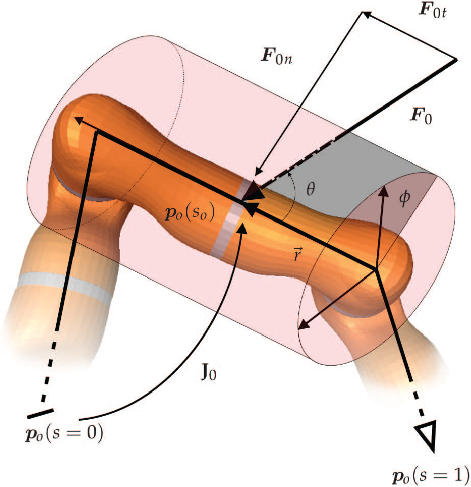
The contact force vector that is acting on a robot link can be represented in a cylindrical coordinate system (see Figure 2), which is aligned with the corresponding robot link backbone. Assuming that the tangential force component is zero, the angle $θ = π / 2$ ). Thus, considering only the normal component $F_{0}_{n}$ of the external force, the force can be defined with two parameters: the amplitude $∥ F_{0}_{n} ∥$ and the direction ϕ:

Figure 2.

The force vector that is acting on the specific segment of the robot can be represented in a cylindrical coordinate system

F_{0}_{n} = ‖ F_{0}_{n} ‖ {[c o s (ϕ), s i n (ϕ), 0]}^{T}

(12)

With this assumption, the dimensionality is $κ = 3$ and $κ = 2$ for the spatial and planar robot cases, respectively.

To estimate the contact point location $p_{0}$ , it is necessary to define the Jacobian matrix $J_{0}$ for the contact point (see Figure 1). To simplify the estimation, we propose to define the contact point location with minimal parameters. As we are dealing with a serial link robot structure, we introduce a new variable, s, which defines the nominal location of point $p_{0}$ along the robot structure (see Figure 2). If the point $p_{0}$ is on the link i, then:

s = \frac{a_{i} + \sum_{k = 1}^{i - 1} l_{k}}{\sum_{i = 1}^{n} l_{k}}

(13)

where $l_{i}$ denotes the link lengths and $a_{i}$ is the distance between joint i and point $p_{0}$ . The variable s has values within the interval $[0,1]$ , where $s = 0$ denotes the robot base and $s = 1$ denotes the robot end-effector.

Using this new variable, we can define the Jacobian $J_{0}$ as a function of s:

J_{o} (s) = J (p_{o} (s))

(14)

which indicates that the Jacobian in the contact point depends upon the contact point position $p_{0}$ and where this position depends upon s. Consequently, the problem of searching for the contact point location $p$ is reduced to a one-dimensional problem of finding the variable s.

Let us denote the estimated external force as $F_{s}$ and the estimated contact point as $p_{s}$ . Then, using Eq. (6), the estimated external torques $τ_{s}$ are:

τ_{s} = J_{o}^{T} (p_{s}) F_{s}

(15)

The problem is how to find the solution for above equation so that $τ_{s}$ are equal to the $τ_{F}$ in Eq. (10). We propose to use optimization methods to find such $τ_{s}$ , that the $∥ p_{o} (s) - p_{s} ∥$ and $∥ F_{0}_{n} - F_{s} ∥$ are minimal.

The estimated external force is represented with its direction and amplitude:

F_{s} = ‖ F_{s} ‖ {\bar{F}}_{s}

(16)

where ${\bar{F}}_{s}$ represents the normalized external force. Note that in the following we denote by $(\bar{\cdot})$ all the variables related to the force ${\bar{F}}_{s}$ .

Estimating the force amplitude is trivial. Let us assume that we know the torques ${\bar{τ}}_{s}$ :

{\bar{τ}}_{s} = J_{o} {(s)}^{T} {\bar{F}}_{s}

(17)

which are caused by the force ${\bar{F}}_{s}$ acting in the same direction as $F_{s}$ . Normalizing ${\bar{τ}}_{s}$ Eq. (17), this can be rewritten as:

{\overset{̌}{\bar{τ}}}_{s} = \frac{{\bar{τ}}_{s}}{‖ {\bar{τ}}_{s} ‖} = J_{o}^{T} (p_{s}) \frac{F i_{s}}{‖ {\bar{τ}}_{s} ‖ {‖ F ‖}_{s}}

(18)

Note that ${\overset{⌣}{\bar{τ}}}_{s}$ is a unit vector in n-dimensional space. Normalizing Eq. (15) and considering that:

\frac{τ_{s}}{‖ τ_{s} ‖} = {\overset{̌}{\bar{τ}}}_{s}

(19)

then by combining Eqs. 15 and 18, the force amplitude can be calculated as:

‖ F_{s} ‖ = \frac{‖ τ_{s} ‖}{‖ {\bar{τ}}_{s} ‖}

(20)

Therefore, it is not necessary to include the external force amplitude calculation in the optimization process, as explained later.

The contact is now characterized with the scalar s defining the location of the contact point on the robot structure and the direction (angle) of the contact force vector ϕ. Consequently, the dimensionality of the problem is reduced to $κ = 2$ for the spatial case and to $κ = 1$ for the planar case.

We propose to solve Eq. (10) by using constrained nonlinear optimization methods. Note that, because of the torque normalization utilized during the calculation of the contact force amplitude, the total number of n equations is reduced by one.

Let us explain this using a simple example. If the external force is acting in such a way that it influences only one joint, the torque in this joint can be calculated as $τ = \vec{r} (s) \times F$ , where one known variable $(τ)$ is on the l.h.s while on the r.h.s are two unknown variables s (representing the lever arm) and the force amplitude $∥ F ∥$ . Obviously, multiple solutions exist. Actually, it is not even important to know the exact location s – we can select it arbitrarily and then calculate the corresponding force amplitude. It can easily be shown that any action we perform based on this force will be the same regardless of the selected location s.

Such a situation always arises when estimating the contact force that is acting on the first segment of the robot, or in such a way that it influences only one robot joint. In this case, some additional sensory equipment (like tactile skin or a camera, etc.) is necessary if we want to determine the contact location exactly.

4. Optimization process

In general, the constrained optimization problem is a problem of solving n nonlinear equations with κ unknowns, which are constrained. If $n < κ$ , the system is underdetermined and it has infinitely many solutions. If the number of equations and unknowns is the same, $n = κ$ , then the system has one solution. In the case where there are more equations than unknowns, $n > κ$ , the system is overdetermined and has a solution only when there are enough linearly dependent equations or when only an approximate solution can be found minimizing some criterion.

The constrained optimization problem is the process of minimizing an objective function $f (x)$ with respect to some variables $x$ :

\begin{matrix} \min_{x} f (x) \\ subject to g_{i} (x) = c_{i} & i = 1, \dots, n \\ h_{j} (x) > = d_{j} & j = 1, \dots, m \end{matrix}

(21)

The goal of the optimization procedure is to find the best approximate solution and the most popular criterion is to select for the objective f a norm $∥ \cdot ∥$ . Let the objective function value $f^{*}$ be:

f^{*} = ‖ τ_{F} - τ_{s} ‖

(22)

where $τ_{F}$ and $t q s$ are the measured and estimated torques, respectively. Then, the value of the objective function is minimal when the difference between the estimated external torques and the measured external torques is minimal. Rewriting the measured external torques into the form:

τ_{F} = ‖ τ_{F} ‖ (\frac{τ_{F}}{‖ τ_{F} ‖})

(23)

and the estimated external torques into the form:

τ_{s} = {‖ F ‖}_{s} (J_{s, p}^{T} \frac{F_{s}}{‖ F_{s} ‖})

(24)

and using the same reasoning as in Eqs. (16), (17) and (20), we can rewrite Eq. (24) as:

τ_{s} = ‖ τ_{F} ‖ \frac{{\bar{τ}}_{s}}{∥ {\bar{τ}}_{s} ∥}

(25)

Then, the objective function Eq. (22) is:

f^{*} = ‖ τ_{F} ‖ ‖ \frac{τ_{F}}{‖ τ_{F} ‖} - \frac{{\bar{τ}}_{s}}{‖ {\bar{τ}}_{s} ‖} ‖

(26)

It is obvious that in order to minimize $f^{*}$ we must minimize only the second part of Eq. (26). Thus, the final objective function f is defined as:

f = ‖ \frac{τ_{F}}{‖ τ_{F} ‖} - \frac{{\bar{τ}}_{s}}{‖ {\bar{τ}}_{s} ‖} ‖

(27)

Note that by using this objective function we minimize the angle between two unit vectors in a n -dimensional space, i.e., the estimated external force $F_{s}$ and position $p_{o} (s)$ cause such joint torques that the relative effect for the particular joint torque components $τ_{s}_{i}$ , $i = 1, \dots, n$ is as in the measured external torques $τ_{F}$ .

We can define a state vector of the unknown variables $x$ for the optimization process as:

x = [s, φ], φ = \frac{ϕ}{2 π}

(28)

for the spatial robot, and:

x = [s]

(29)

for the planar case. In both cases, the states are constrained:

0 \leq s \leq 1 and 0 \leq ϕ \leq 1

(30)

In our case, we have only the inequality constraints:

l \leq x \leq u

(31)

where $l$ and $u$ are the lower and upper bounds for the variables $x$ .

The objective function Eq. (27) is a multi-variable function with simple bounds. The result of the minimization problem consists of the values of the state vector, which lead to the minimum value of the objective function. By definition, unless the objective function and the feasible region are convex in the minimization problem, there may be several local minima. As the objective function Eq. (27) is a non-convex function, several local minima are likely to exist, each on different segments of the robot.

Many of well-known optimization algorithms proposed for solving non-convex problems are not capable of making a distinction between local and global optimal solutions, and they treat the local optimal solutions as the actual solutions to the problem. Therefore, it is necessary to use a global optimization method that finds the global minimum of the objective function.

Since global optimization methods search for the global minimum over the entire constrained space they are time consuming. However, considering the fact that once the robot is in contact with the environment, the contact force (location and direction) does not change significantly during one time step, i.e., we assume a continuous force and location. Thus, once we obtain the solution, the search interval Eq. (30) can be narrowed to the neighbourhood of the previous solution for the next time steps:

\begin{matrix} s (t_{k}) = s (t_{k - 1}) \pm δ_{s} \\ φ (t_{k}) = φ (t_{k - 1}) \pm δ_{φ} \end{matrix}

(32)

where k denotes the time instance, while $δ_{s}$ and $δ_{φ}$ define the neighbourhood. As it is not likely that in this narrower search space more minima exist, it is appropriate to use local optimization methods, which are in general faster than global ones.

In our paper for the global optimization method, the DIRECT algorithm [17, 18] was used, while the FMINCON algorithm [19] was used in the local optimization method.

During the first step of the optimization process, the DIRECT algorithm estimates the function value in the set of points sampled by the algorithm, which are scattered over the constrained interval Eq. (30). The DIRECT algorithm converges on the global optimal function value if the objective function is continuous or at least continuous within the neighbourhood of a global optimum. The convergence of the algorithm is shown in [17]. During the next steps, the value obtained from the previous global optimization search is used as the initial value for the local optimization search during the reduced constrained interval Eq. (32).

5. Experimental and simulation results

To evaluate the proposed estimation of external forces, we first show the simulation results for a planar robot manipulator, after which we give the simulation results for a seven-DOF robot. Finally, we implemented the proposed algorithm on a KUKA LWR robot and now give some experimental results.

5.1. Contact location estimation on a four-DOF planar robot

A planar robot was modelled in the MATLAB/Simulink environment using the MATLAB Planar Manipulators Toolbox [20]. As described in the section 3, the dimensionality of the contact search problem on a planar robot is reduced to $κ = 1$ . The result of the optimization process is the location at which the contact force acts upon the robot structure. The contact force amplitude is estimated after the optimization process, as described in Eq. (20). Since the contact is assumed to be frictionless, only the normal component of the force is estimated.

The state vector (i.e., variables that are the subject of the nonlinear optimization) is Eq. (29), with the corresponding constraints Eq. (30).

In the simulation, a planar robot with four revolute joints and link-lengths $l_{i} = 1$ , $i = 1, \dots,4$ , was used. Meanwhile, in its initial configuration $q_{0}$ , $q_{o} = [0,1, - {2,1]}^{T}$ , an external contact force with amplitude $∥ F_{0} ∥ = 2 N$ was acting upon the robot structure at the different locations $p_{0} (s_{i})$ , where:

s_{i} = {0.125, 0.3750, 0.6250, 0.8750}

(33)

The external joint torques were calculated from the known force and contact location, as in Eq. (10). Some white noise with a signal-to-noise ratio of 20 was added to the estimated torque signal. The configuration of the planar robot with contact forces acting at different locations $s_{i}$ is shown in Figure 3.

Figure 3.

The contact force vector acting at different locations on the robot structure (N.B. the black arrow indicates the external force; the yellow arrow indicates the estimated force)

The estimated contact force is defined as:

F_{s} = ‖ F_{s} ‖ [\begin{matrix} c o s (ϕ_{i}) \\ s i n (ϕ_{i}) \end{matrix}] ϕ_{i} = \frac{π}{2} + \sum_{j = 1}^{L (i)} q_{j}

(34)

where $L (i)$ denotes the link number where the point $p_{s} (s_{i})$ is assumed. Note that the direction of the force ϕ is assumed to be perpendicular on the robot segment.

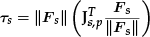
The objective function values in the optimization using the DIRECT algorithm for the selected external forces are shown in Figure 4. It can be seen from the figure that when the contact force is acting upon the first segment of the robot (i.e., the contact point at $s_{1}$ ), the optimization search is unable to find a unique solution. The reason is that when $L (i) = 1$ , Eq. (10) reduces to two linear, dependent equations.

Figure 4.

Objective function values for different contact point locations (N.B. the global minimum is marked with a blue circle; the intermediate results of the optimization algorithm are marked with an empty diamond)

Once the optimization process is over and the contact point location $p_{s} (s_{i})$ is known, the estimated contact force amplitude $∥ F_{s} ∥$ is calculated as described by Eq. (20).

5.2. Seven-DOF robot dynamic model simulation

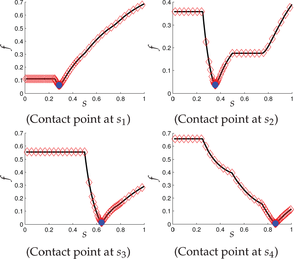
In the next simulation, we used a seven-DOF robot with the same structure as the KUKA LWR robot. The robot was modelled in the MuJoCo simulation environment [21], which enables the modelling and simulation of multi-body dynamic systems with contacts. The robot segments were modelled as cylinders and a frictionless contact model was used. As before, we considered all the approximations mentioned in section 3. The simulation setup and control scheme are shown in Figure 5 and 6.

Figure 5.

Control scheme for the contact estimation algorithm of a seven-DOF robot in the MuJoCo simulation environment

Figure 6.

Model of a seven-DOF robot in MuJoCo

The state vector $x$ for the optimization process was selected as in Eq. (28) and with constraints as in Eq. (30).

While moving, the robot collided with an obstacle in the robot workspace and slid along it. This contact created contact forces which influenced the robot joint torques. The resulting external torques were estimated from the measured joint torques using the known dynamic model of the robot as described in Eq. (5).

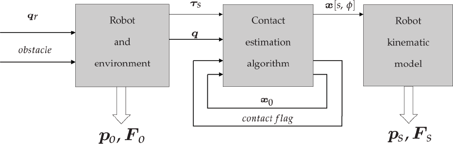
The Figure 7 shows the plots of the objective function values for two instances of the optimization procedure. During the first (initial) step, the result is obtained using the global optimization method based on the DIRECT algorithm, which searches for the result throughout the entire constrained space. The result from this step is then used as an initial value for the search with the local optimization method FMINCON on the narrowed interval Eq. (32), where the $δ_{s}$ and $δ_{φ}$ were chosen as:

Figure 7.

The objective function values for a seven-DOF robot: a) optimization with the DIRECT algorithm during the first step; b) optimization with the FMINCON algorithm during the next steps

\begin{array}{r} δ_{s} = 0.1 \\ δ_{φ} = \frac{1}{8} \end{array}

(35)

The external force is modelled as given by Eq. (12). The result of the optimization process was the normalized distance from the robot base s and the contact force direction φ. The results of the optimization can be seen in Figure 8.

Figure 8.

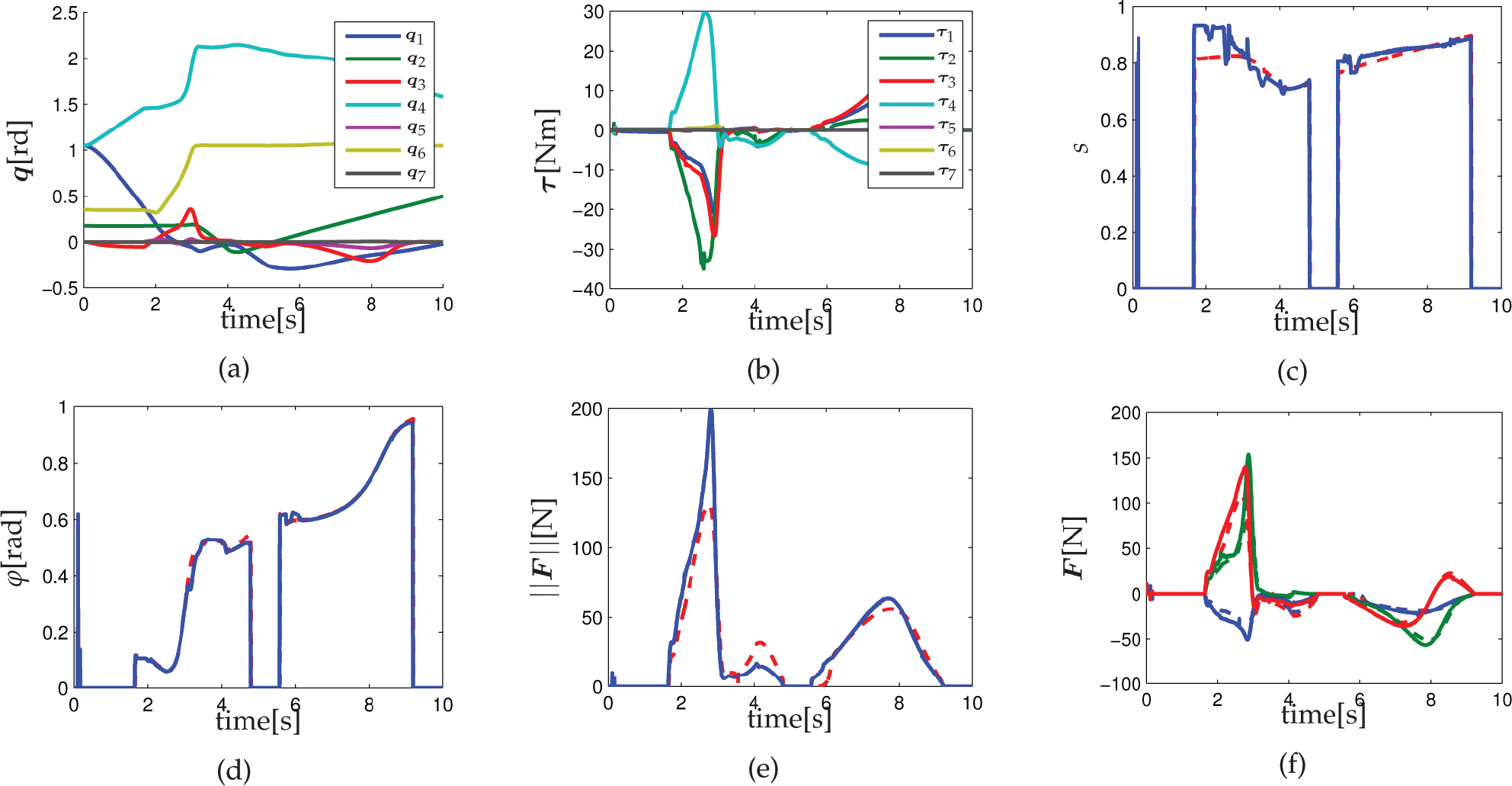
Simulation results for the seven-DOF robot colliding twice with the obstacle (at $t = 1.6 s$ and $t = 5.5 s$ ). The figure shows: (a) joint positions; (b) external joint torques (estimated from the measured joint torques and the dynamic model); (c) and (d) the values of the state vector; (e) the contact force amplitude; (f) the contact force vector (N.B. the estimated values are marked with a solid line, while the actual values are marked with a dashed line).

5.3. Time analysis of the optimization algorithm

The time analysis of the optimization algorithm was made on the simulation environment described in section 5.2. The evaluation time of the optimization algorithm depends upon the number of steps necessary to find the solution at the desired level of accuracy, which in our case is 3% for the position variable s and force direction angle ϕ. Note that the required accuracy depends upon the needs of the application in question. For example, when using the contact force information in combination with obstacle avoidance, practical experience has shown that an accuracy of about 3% is sufficient.

During each iteration step of the optimization routine, there are several function evaluations which require computational time. As expected, the total computational time increases with the number of iterations. As described in section 4, the main problem is to estimate the location at which the external force acts upon the robot structure. As we do not have any prior information as to the location of the external force, and since the system is highly nonlinear, we propose that the global optimization method be used in the first search (i.e., when the contact occurs). The use of the global optimization is necessary to find the global solution and in order to avoid ending in a local optimum. Thus, during this step the DIRECT algorithm finds the global optimum. It was experimentally evaluated that a minimum of 15 iterations are needed using the global optimization algorithm in order to get an adequate solution. Of course, it is possible to reduce the number of iterations, but consequently the accuracy and the continuity of the result are also reduced. Afterwards, and assuming the continuity of the position of the force location, we propose to use a local optimization method with initial values from the previous step. Since the local optimization method requires less function evaluation in obtaining the same accuracy for the result as the global optimization method (and is therefore faster), the usage of the combined optimization method is reasonable.

The results of the time analysis are shown in Figure 9. It is easy to see the difference between the timing, the number of function evaluations and the accuracy of the global optimization method using five and 15 iterations. Next, using the combined optimization method, we can achieve the same accuracy but with fewer iterations as with the global method using 15 iterations.

Figure 9.

Time analysis of the algorithm: a) the number of objective function evaluations under the optimization method; b) the evaluation time for the optimization method; c) the contact location error; d) the contact force direction angle error (N.B. the values obtained with the DIRECT algorithm, using five and 15 iterations, are marked with dotted and dashed lines, respectively, the values of the combined optimization method are marked with a solid line, and the vertical dashed lines with $t_{1}$ and $t_{2}$ represent the start and end of the contact, respectively).

Of course, this approach has the drawback that, during the first step, it needs more function evaluations (i.e., more time) wherever the global optimization method is used. In the next steps, the degree of computational complexity and the calculation times are comparable to the five-iteration global optimization method. From Figure 9 b), we can conclude that the use of the proposed method for the estimation of the contact force and location is practical and suitable in those applications which do not require an acquisition rate faster than 30 Hz. Note, that the frequency of the acquisition could be higher, but then the accuracy would be reduced. The error on figures c) and d) was calculated as the difference between the real values and the estimated values during the time interval between $t_{1}$ when the contact occurs and the $t_{2}$ when the robot is no longer in contact.

5.4. Experimental evaluation of the contact point detection algorithm

The algorithm of the external force and contact point estimation was experimentally evaluated on a KUKA LWR seven-DOF robot arm. The details of the robot system setup are described in [22] and shown in Figure 10.

Figure 10.

KUKA LWR robot system overview: 1) LWR robot; 2) teach pendant KCP 3); robot controller with FRI; 4) connection controller/pendant; 5) connection controller/robot; 6) FRI-xPC server; 7) client controller; 8) connection FRI-xPC/controller; 9) connection FRI-xPC/client

The robot, in position control mode [13], was controlled using a controller implemented in MATLAB/Simulink running on a client computer, which was connected to the robot controller by the Fast Research Interface (FRI). The FRI provided information about the external joint torques from the joint torque sensors at a frequency rate of 1 kHz, and which was acquired by the computer running MATLAB/Simulink at a frequency rate of 100 Hz while the contact estimation algorithm was running at 30 Hz. 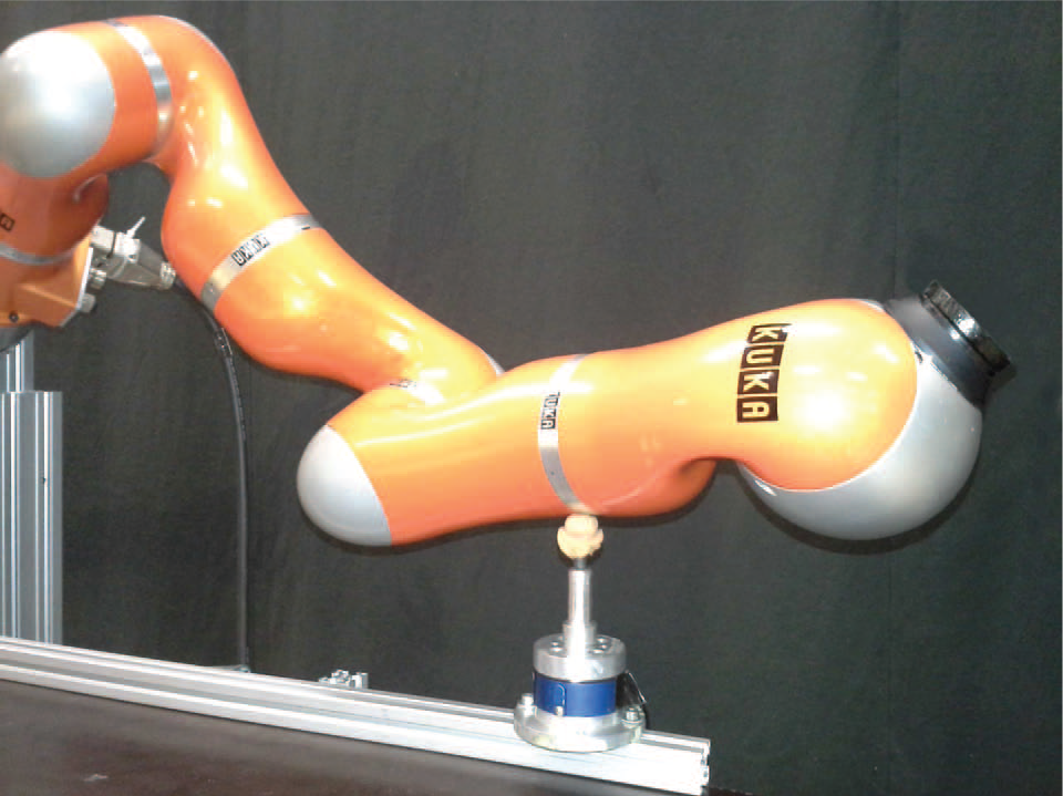The trajectory for moving the robot was predefined in such a way that a particular point on the robot structure at $s = 0.7683$ collided with a JR3 multi-axis force-torque sensor placed at a fixed position, which produced the external joint torques. The experimental setup is shown on Figure 11.

Figure 11.

The experimental setup for testing the contact point detection algorithm with a KUKA LWR robot arm and a JR3 multi-axis force-torque sensor

The state vector x and the constraints were selected as in the previous experiment. The external force was modelled as given by Eq. (12). The simulation results can be seen in Figure 12.

Figure 12.

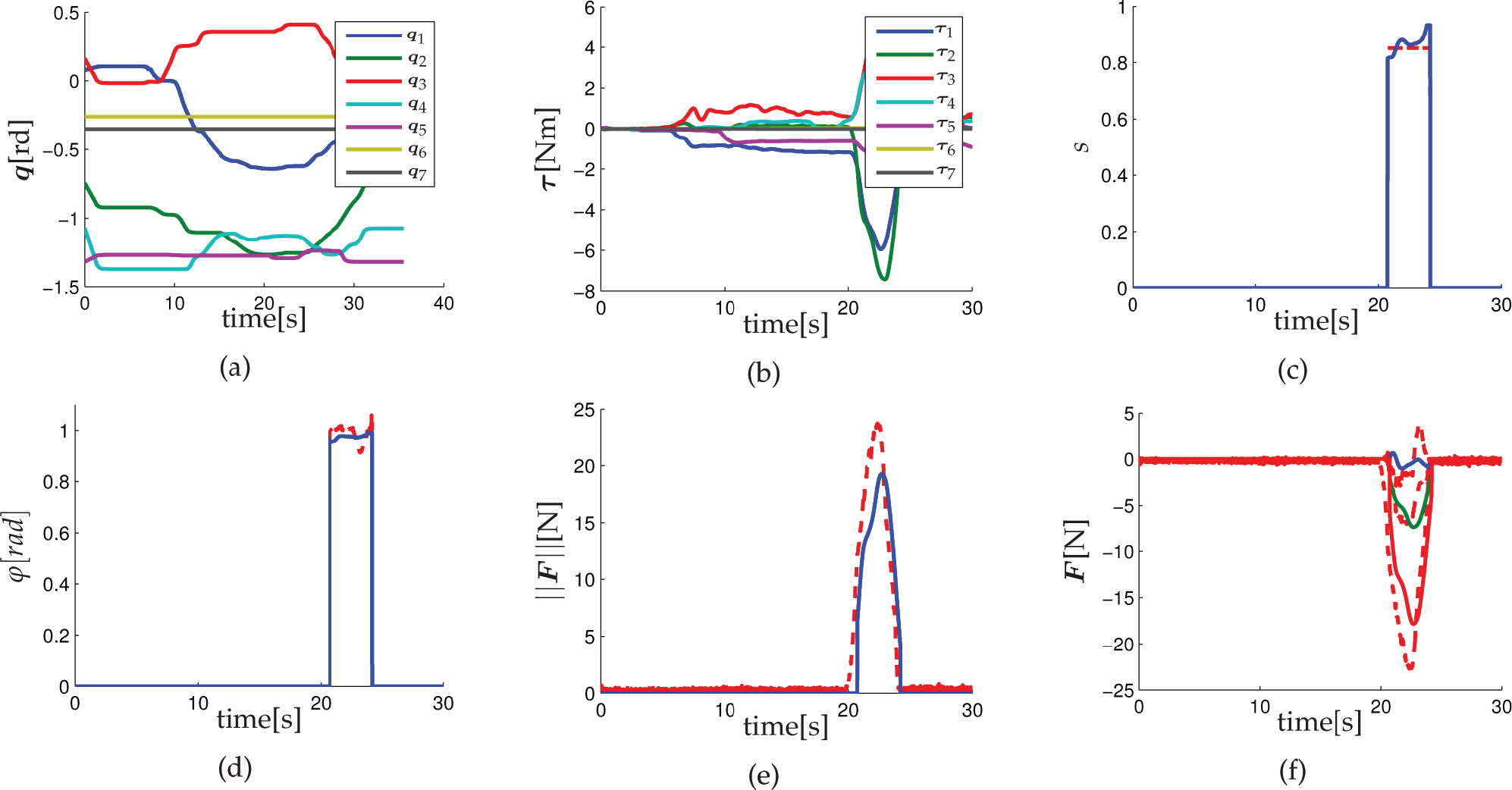
Experimental results using KUKA LWR when a contact with an obstacle occurs during motion: (a) joint positions; (b) external torques obtained from FRI; (c) and (d) values of the state vector; (e) contact force amplitude; (f) contact force vector (N.B. the estimated values are marked with a solid line, while the actual values are marked with a dashed line)

In the second experiment, we evaluated the contact estimation method when the force acts at different locations and from different directions. Here, the robot had a fixed configuration, not moving, and the human operator was holding a JR3 multi-axis force/torque sensor and touched the robot at different points on the robot surface. Since the body of the robot is almost cylindrical, the robot body was approximated with backbone lines, as described in section 3, and therefore the contact points on the robot surface could be approximated with points on these lines. The contact points $p_{0} (s_{h, i})$ were at normalized locations:

\begin{array}{l} s_{h, i} & = & {0.1316,0.2632,0.3480,0.4329,0.5178,0.6027, \\ 0.6855,0.7683,0.8510,0.9338} \\ i = 1, \dots,10 \end{array}

(36)

from the base to the end-effector of the robot. The actual and estimated contact points with their estimation error are shown in Figure 13.

Figure 13.

The locations of the contact points on the robot structure and the estimation error at the corresponding contact points (N.B. the arrows represent the direction of the applied contact forces)

As we can see, the accuracy of the estimated locations of the contact points is better when the contacts are closer to the end-effector. This observation is as expected. Because of the selected contact force direction and current robot configuration, while estimating the contact point on the second robot segment the problem Eq. (10) manifests as an underdetermined system, since the torque measurements are available only for one robot joint. Additionally, the noise in the torque measurements and the errors in the dynamic model parameters influence the calculation of the external joint torques. As the Jacobian matrix $J_{0}$ in the contact point (see Eqs. (8) and (10)) is sparser for contact points closer to the robot base, the sensitivity of the estimation of the contact force and the contact position to the external joint torques errors is greater when the contact point is closer to the robot base. At first sight, it seems that something is wrong with the estimated contact position at Point 5 in Figure 13. However, note that the force is acting in such a way that it influences only the second joint. Hence, the system was unable to estimate an accurate contact position (as explained in Section 3).

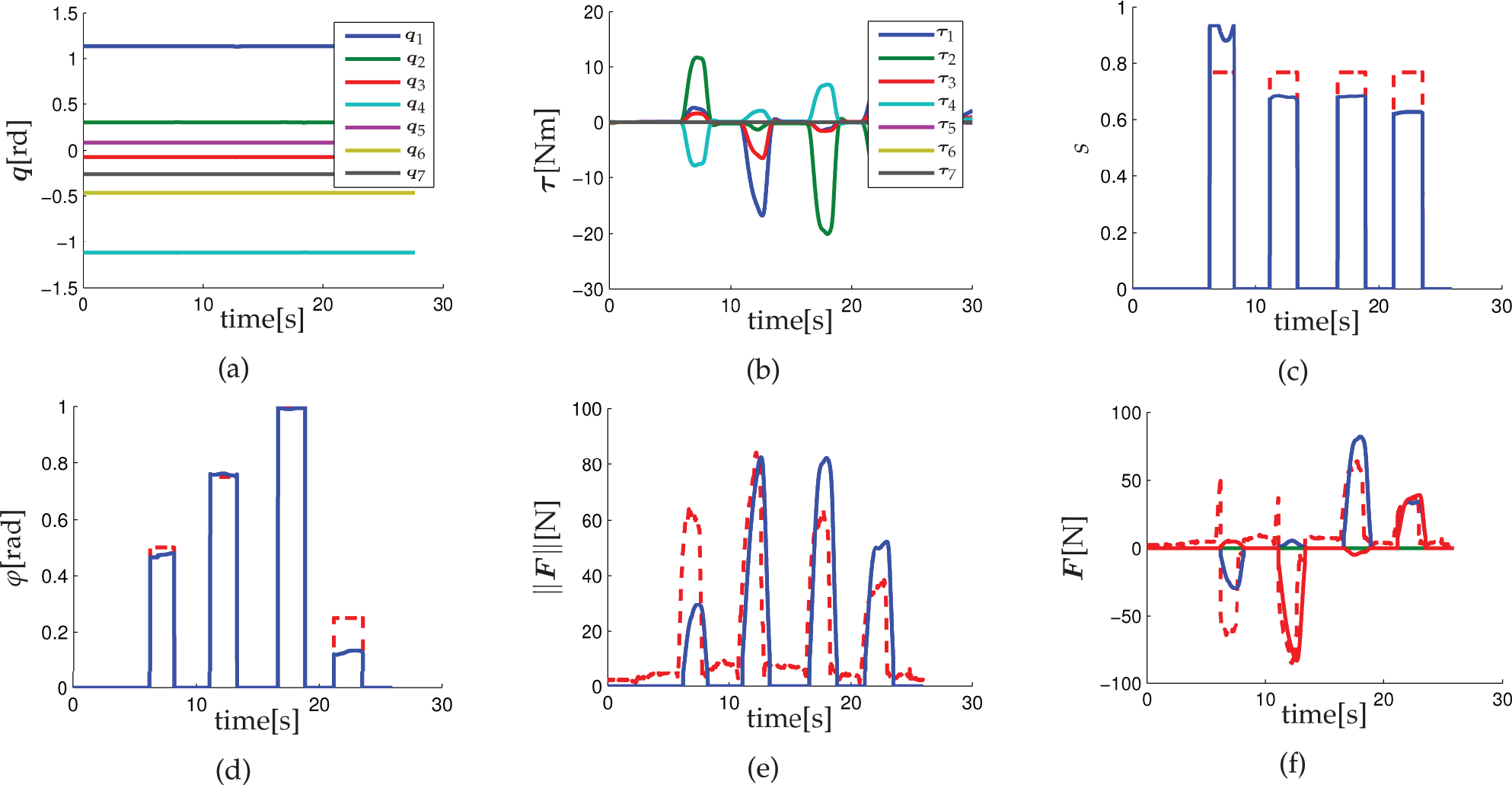
In the third experiment, the robot had the same configuration as in the previous experiment and was not moving. The proposed algorithm estimated the contact information while the contact force acted from different directions. Similar to the previous experiment, the human operator applied a force from four different directions while holding a force sensor (with an offset angle $\sim π / 2$ ) around the point $p_{0} (s_{7})$ (marked with 7 in Figure 13). The results are shown in Figure 14.

Figure 14.

Experimental results for the external force acting at one point from different directions: (a) the joint positions; (b) the external torques obtained from FRI; (c) the contact point position; (c) and (d) the values of the state vector; (f) the contact force vector (N.B. the estimated values are marked with a solid line, while the actual values are marked with a dashed line)

6. Conclusion

The paper proposed a method for estimating the external force acting on the body of a robot (i.e., the location of the application point and the external force) using information about the part of joint torques due to the external forces. The estimation is limited to robots with cylindrically-shaped links. The problem of estimating the external force based on joint torques is not easy, since the contact force may arise from a wide variety of contact situations. Using a combination of the global and local optimization methods, it was possible to estimate the contact point location and contact force, corresponding to the measured external joint torques caused by the external force from the contact. With some approximations, the dimensionality of the problem is greatly reduced and the methods are feasible for use with real robots. Note that the algorithm can be extended to a more general case using a more complex problem definition of the state vector variables and a greater number of contacts, etc. However, this results in the increasing complexity of the optimization.

The algorithm was verified by simulations and experiments. The results show that with the proposed method – and under some assumptions – it is possible to estimate the external force and locate the position of the contact point, and that this can also be done in real-time with a real robot. Of course, its practical applicability depends upon the particular usage of the estimated external force.

References

Hogan

Neville

. Impedance control: An approach to manipulation: Part 3 applications. J. Dyn. Sys., Meas., Control, 107(1):17–24, 1985.

Tsuji

Takahashi

Ito

Stifter

, and Lenaric

Multi-point compliance control for redundant manipulators. Advances in Robot Kinematics. Springer-Verlag, 1991.

Tsuji

Jazidie

, and Kaneko

Multi-point impedance control for redundant manipulators. Systems, Man, and Cybernetics, Part B: Cybernetics, IEEE Transactions on, 26(5):707–718, 1996.

Hwang

S K

and Hwang

H Y

. Development of a tactile sensing system using piezoelectric robot skin materials. Smart Materials and Structures, 22(5):055004, 2013.

Cannata

Giorgio

Maggiali

Metta

, and Sandini

An embedded artificial skin for humanoid robots. In Multisensor Fusion and Integration for Intelligent Systems, 2008. MFI 2008. IEEE International Conference on, pages 434–438, 2008.

Albu-Schaffer

Eiberger

Grebenstein

Haddadin

Ott

Wimbock

Wolf

, and Hirzinger

Soft robotics. Robotics Automation Magazine, IEEE, 15(3):20–30, 2008.

Petrovskaya

Park

Jaeheung

, and Khatib

Probabilistic estimation of whole body contacts for multi-contact robot control. In Robotics and Automation, 2007 IEEE International Conference on, pages 568–573, 2007.

Phong

Le Dinh

Choi

Junho

, and Kang

Sungchul

. External force estimation using joint torque sensors for a robot manipulator. In Robotics and Automation (ICRA), 2012 IEEE International Conference on, pages 4507–4512, 2012.

Van Damme

Beyl

Vanderborght

Grosu

Van Ham

Vanderniepen

Matthys

, and Lefeber

Estimating robot end-effector force from noisy actuator torque measurements. In Robotics and Automation (ICRA), 2011 IEEE International Conference on, pages 1108–1113, 2011.

10.

Eberman

Brian S.

and Kenneth

Salisbury J.

Determination of manipulator contact information from joint torque measurements, 1990.

11.

De Luca

and Mattone

Sensorless robot collision detection and hybrid force/motion control. In Robotics and Automation, 2005. ICRA 2005. Proceedings of the 2005 IEEE International Conference on, pages 999–1004, 2005.

12.

Sadeghian

Keshmiri

Villani

, and Siciliano

Null-space impedance control with disturbance observer. In Intelligent Robots and Systems (IROS), 2012 IEEE/RSJ International Conference on, pages 2795–2800, 2012.

13.

Schreiber

Stemmer

, and Bischoff

The fast research interface for the kuka lightweight robot. In ICRA 2010 Workshop on Innovative Robot Control Architectures for Demanding (Research) Applications, pages 15–21, 2010.

14.

Aghili

Farhad

. Joint Torque Sensory in Robotics. Industrial Robotics: Programming, Simulation and Applications, Low Kin Huat. InTech, 2006.

15.

Bicchi

Antonio

Kenneth

Salisbury J.

, and Brock

David L.

Contact sensing from force measurements. International Journal of Robotics Research, 12:249–262, 1993.

16.

Salisbury

Jr.

Interpretation of contact geometries from force measurements. In Robotics and Automation. Proceedings. 1984 IEEE International Conference on, volume 1, pages 240–247, 1984.

17.

Jones

D. R.

Perttunen

C. D.

, and Stuckman

B. E.

Lipschitzian optimization without the lipschitz constant. J. Optim. Theory Appl., 79(1):157–181, October 1993.

18.

Björkman

Mattias

and Holmström

Kenneth

. Global optimization using the direct algorithm in matlab. In in Matlab. Advanced Modeling and Optimization 1(2), pages 17–37, 1999.

19.

Matlab fmincon – find minimum of constrained nonlinear multivariable function. www.mathworks.com/help/optim/ug/fmincon.html. Accessed on 06 Jan 2014.

20.

Žlajpah

Leon

. Simulation of n-r planar manipulators. Simulation Practice and Theory, 6(3):305–321, 1998.

21.

Todorov

Erez

, and Tassa

Mujoco: A physics engine for model-based control. In Intelligent Robots and Systems (IROS), 2012 IEEE/RSJ International Conference on, pages 5026–5033, 2012.

22.