Sage Journals: Discover world-class research

Abstract

This paper presents an algorithm to remove fog from a single image using a Markov random field (MRF) framework. The method estimates the transmission map of an image degradation model by assigning labels with a MRF model and then optimizes the map estimation process using the graph cut-based α-expansion technique. The algorithm employs two steps. Initially, the transmission map is estimated using a dedicated MRF model combined with a bilateral filter. Next, the restored image is obtained by taking the estimated transmission map and the ambient light into the image degradation model to recover the scene radiance. The algorithm is controlled by just a few parameters that are automatically determined by a feedback mechanism. Results from a wide variety of synthetic and real foggy images demonstrate that the proposed method is effective and robust, yielding high-contrast and vivid defogging images. In addition to image defogging, surveillance video defogging based on a universal strategy and the application of a transmission map are also implemented.

Keywords

Foggy Image Defogging Markov Random Field Label Assignment Transmission Map

1. Introduction

Image defogging is an important issue in the field of computer vision. There are many circumstances in which defogging algorithms are needed, such as automatic monitoring systems, automatic guided vehicle systems, outdoor object recognition and visual navigation in low visibility environments, etc. However, the quality of images taken in foggy weather conditions is easily undermined by the aerosols suspended in the medium, which have an effect on the image such that the contrast is reduced and the surface colours become faint. Such degraded images often lack visual vividness and offer a poor view of the scene contents. The goal of defogging algorithms is to recover the details of scenes from foggy images. Since the process of removing fog from an image depends on the depth of the scene, the essential problem that must be solved for most image defogging methods is scene depth estimation. This is not trivial, and requires prior knowledge.

In this paper, we propose a new method that can produce a good defogging effect for various foggy images. The main motivation of this research is to improve the visual quality of images for the bulk of automatic systems and outdoor photos taken in poor weather conditions. For example, in foggy weather, the quality of images captured by a classic in-vehicle camera is drastically degraded, which makes current in-vehicle applications reliant on such sensors very sensitive to weather conditions. An in-vehicle vision system should take fog effects into account if it is to be more reliable. A solution is to remove fog effects from the image beforehand. This is also the case for other applications, such as surveillance, intelligent vehicles, remote sensing and aerial photography, etc. Therefore, restoring foggy images is highly desirable in both computer vision applications and consumer photos. Usually, computer vision algorithms assume that the input image characterizes the scene radiance. The performance of vision algorithms (e.g., feature detection, filtering, object recognition and photometric analysis) will inevitably suffer from the biased, low-contrast scene radiance. Removing fog can significantly increase the visibility of the scene and correct the colour shift caused by the ambient light to make the vision algorithms more effective and the appearance of foggy photos more pleasing. In this paper, the proposed defogging method combines the MRF model with transmission map (scene depth) estimation, and the graph-cut based α-expansion method is used here to optimize the map estimation process. This provides a new way to solve the image defogging problem. The main contribution of this paper can be described as follows:

- A novel MRF-based method is proposed which applies an optimization library to estimate a transmission map. Experiments on both synthetic images and real-world images show the effectiveness of the proposed method. Compared with existing defogging methods, the proposed algorithm can remove fog more thoroughly without producing any halo artefacts, and the colour of the restored images is natural in most cases.

- We extend our proposed method to foggy video applications using a universal strategy, which greatly improves computational efficiency and enhances the visual effect. The application of our transmission map, such as fog simulation, is also implemented based on the estimated transmission map.

- The adaptive adjustment of the algorithm's parameters using a defogging effect measurement index is realized in this paper. Thus, a static, open-loop parameter estimation issue is transformed into a dynamic parameter adjustment issue. In addition, the performance of the defogging algorithms is effectively measured using appropriate qualitative and quantitative evaluations.

The organization of this paper is as follows. We begin by reviewing existing works on image defogging. In Section 3, we introduce the MRF model and the outdoor geometry of a foggy image. In Section 4, we propose a defogging algorithm based on the MRF model. In Section 5, we extend our algorithm to video applications and our transmission map is also presented. In Section 6, we present some experimental results. Finally, in Section 7, we make some concluding remarks.

2. Previous Works

Given the importance of defogging algorithms, many studies on defogging have been conducted. Previous defogging research can be divided into two categories: image enhancement methods and image restoration methods [1]. Image enhancement methods tend to increase the dynamic range and contrast of images degraded by fog. Classic image enhancement algorithms include histogram equalization and a Retinex algorithm. Image restoration methods cover the intrinsic luminance of an object using additional information or prior information. Representative algorithms include the dark channel algorithm [2] and the fast filter algorithm [3]. The dark channel algorithm [2] is recognized as one of the most effective ways to remove fog. The algorithm estimates the transmission map of each patch as the minimum colour component within that patch and employs a soft matting algorithm to refine the map. The fast filter algorithm [3] has been proven to be faster than most other algorithms for outdoor scenes. The algorithm uses a fast median filter to infer the atmospheric veil and further estimate the transmission map. The main advantage of this method is its speed. However, The defogging algorithm in [2] is based on an image prior-dark channel prior, which is a kind of statistics of haze-free outdoor images, and the dark channel prior will be invalid when the scene objects are inherently similar to the ambient light and no shadow is cast on them; in addition, the defogging method in [3] is unable to remove the fog between small objects and the colour of the scene objects is unnatural for some situations.

Graphical models (GMs) are probabilistic models combining probability with a graph, and comprise an important means for solving this problem. Such models can be divided into two categories: directed graphs and undirected graphs. Generally, a directed GM is a Bayesian network (BN) when the graph is acyclic, meaning there are no loops in the directed graph. The relationships in a BN can be described by local conditional probabilities [4]. In [5, 6], a Bayesian defogging method that jointly estimates the scene albedo and depth from a single foggy image is introduced by leveraging their latent statistic structure. The undirected graph refers to a MRF. Since a MRF is undirected and may be cyclic, it can represent certain dependencies that a BN cannot, providing a new means for image defogging due to the dependencies existing between the neighbouring pixels. The defogging algorithm in [7] is based on the observation that the surface Lambertian shading factor and the scene transmission are locally independent. Thus, the fog can be separated from the scene. Then, a Gaussian MRF is used to smooth the intensity value of the transmission map. In [8], a cost function is developed within the framework of MRF to enhance the visibility of images. However, the results obtained by this method tend to have larger saturation values than those in the actual clear-day images. In [9], scene geometry and the α-expansion optimization technique are employed to improve the robustness of a single image dehazing algorithm. Recently, image defogging based on the MRF model has made significant progress [10 –12]. In [10], the image defogging problem is decomposed into two steps: first, the atmospheric veil is inferred using a dedicated MRF model, and second the restored image is estimated by minimizing another MRF energy which models the image defogging in presence of noisy inputs. In this MRF model, the flat road assumption is introduced to achieve better results on road images. In [11], a MRF model for both stereo reconstruction and defogging problems is combined into a unified MRF model to take advantage of both stereo and atmospheric veil depth cues. Thus, the stereo reconstruction and image defogging of daytime fog can be solved using the new MRF model. In [12], a multi-level depth estimation method based on a MRF model is presented for image defogging. The method integrates the characteristics of a dark channel prior into the MRF model in order to estimate an accurate depth map. The MRF is applied, here, to label the depth level in adjacent regions to compensate for wrongly estimated regions. The textures in the scene are the critical element, serving as the smoothing term in the MRF model. These fog removal algorithms are the most representative of MRF defogging methods, and they are all physically sound. However, the colour and the profile of the scene objects can sometimes look unnatural for the defogged results. To solve the problem, we introduce an image assessment index to the MRF model to optimize the parameters of the proposed method. Thus, visually pleasing defogging results can be obtained.

3. Background

3.1 Markov Random Fields

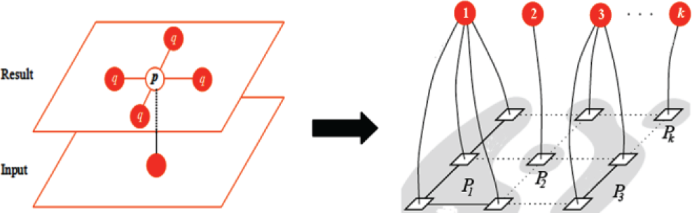
Many vision problems can be solved naturally using the MRF technique. MRF theory is a branch of probability theory for analysing the spatial or contextual dependencies of physical phenomena. It is often used in visual labelling to establish the probabilistic distributions of interacting labels. Here, we use an MRF to estimate the transmission map in an image degradation model. It is an undirected graph, and adjacent nodes are connected to determine the depth of a real scene [12]. We associate a hidden layer with the dense level of fog and an observation layer with the initial transmission map, and then a MRF model is added to a cost function, such that:

E (f) = \sum_{p ∊ P} D_{p} (f_{p}) + \sum_{(p, q) ∊ N} V_{p, q} (f_{p}, f_{q}),

(1)

In (1), f = {f_p | p ∊ P} is a labelling of image P, f_p is the label of pixel p in image P, and f_p = {1,2,3, …, k}. In addition, q is the neighbour of p, N is the set of pairs of pixels defined over the standard four-connection neighbourhood, E(f) is for minimizing the sums of two types of terms, and the first term D_p(·) is a data function. The smaller the difference between a pixel and its label, the smaller D_p(·) will be. D_p(·) penalizes a label f_p assigned to pixel p if it is too different from the observed data I_p. The second term V_p,q(·) is a smoothing function (or a ‘discontinuity-preserving’ function) [13, 14]. The smaller the difference among the labels of the pixels in set N, the smaller V_p,q(·) will be. V_p,q(·) encourages the integrity of an image by penalizing two neighbouring labels f_p and f_q if they are too different. The choice of V_p,q(·) is a critical issue, and in the proposed defogging method we apply the outdoor geometry to obtain this term. With the smoothing term, the saturated colours at each pixel can be computed with reasonable smoothing. Thus, for the transmission map estimation, the data function represents the probability of pixel p having a transmission association with label f_p. The smoothing function encodes the probability whereby neighbouring pixels should have a similar depth. A graph cut is used here to minimize the energy function of the MRF. The method transforms an image represented by a set of pixels into a graph with an augmented set of nodes, and then cuts the graph into different sets. The cuts correspond to some assignment of pixels to labels. If the edge weights are appropriately set based on the parameters of the energy function [see Eq. (1)], a minimum cost cut will be obtained by labelling each pixel according to the minimum value of this energy function. Thus, in finding a cut that has the minimum cost among all cuts, the minimum value of the energy function of the MRF can be obtained and a proper label can be assigned to each image pixel, as shown in Figure 1. Therefore, the graph cut technique transforms the energy minimization problem to an equivalent problem concerning finding an effective way to partition a special graph constructed according to the primal minimization problem into different sets. α-expansion algorithm is used to solve the graph cut problem with good computational performance. For the transmission map estimated using the MRF model, the smaller value of the label on behalf the deeper depth in the scene, while the lager value corresponding to the scene points which near the camera or observer. The relabeling results would constitute the initial transmission map of the proposed method. However, there remains certain redundant details that need to be removed.

Figure 1.

Label assignment by energy minimization

3.2 Outdoor geometry for the foggy image

In this section, we present the outdoor geometry that is used in the transmission map estimation of the proposed algorithm. Light passing through a scattering medium is attenuated and distributed in other directions. This can happen anywhere along the path and leads to a combination of radiances incident towards the camera, as shown in Figure 2.

Figure 2.

Scattering of light by atmospheric particles

Formally, to express the relative portion of light that managed to survive passage along the entire path between the observer and a surface point within the scene, the defined transmission map t_i combines the geometric distance d_i and the medium extinction coefficient β (the net loss from scattering and absorption) into a single variable [15]:

t_{i} = e^{- β d_{i}}

(2)

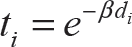
According to (2), the following outdoor geometry is reasonable: assuming that β is constant over the image, the variations in transmission are due to the distance d between the scene point and the camera such that, the greater the distance, the lower the intensity in the transmission map. For most outdoor images, an object which appears closer to the top of the image is usually further away. Thus, the distance along the ground to the object is a monotonically increasing function of the image plane height, which starts from the bottom of image going up to the top. For example, from Figure 3(a) one can clearly see that the distance between the scene point R and the camera is smaller than that between scene point S or T and the camera. In addition, the intensity at point R in the transmission map is higher than that of point S or T, as shown in Figure 3(b). Figures 3(c–d) show the relationship between the height position of the observation point and its distance or intensity in relation to the transmission map.

Figure 3.

The distance and intensity relationship of any scene point. (a) Input foggy image and three scene points. (b) The transmission map for (a) and the scene points. (c) The relationship between the height position of the observation point and its distance. (d) The relationship between the height position of the observation point and its intensity in relation to the transmission map.

4. The Proposed Algorithm

4.1 The algorithm flowchart

Specifically, the proposed algorithm employs three steps in removing fog from a single image. The first one involves computing the ambient light according to the three distinctive features of the sky region. The second step involves the computing of the transmission map with the MRF model and the bilateral filter. The goal of this step is to assign an accurate pixel label using the graph cut-based α-expansion and to remove any redundant details using the bilateral filter. Finally, with the estimated ambient light and the transmission map, the scene radiance can be recovered according to the image degradation model. The flowchart of the proposed method is depicted in Figure 4.

Figure 4.

Flowchart of the algorithm

4.2 Ambient light and transmission map estimation

The presence of aerosols in the lower atmosphere means that the light may scatter and be absorbed while travelling through the medium [16]. This can happen anywhere along the path, and it can lead to a combination of radiances incident towards the camera. The image degradation model that is widely used to describe the formation of foggy images is as follows [2]:

I (x) = J (x) t (x) + A (1 - t (x))

(3)

where I(x) is the observed intensity corresponding to the pixel x=(x, y), the input foggy image J(x) is the scene radiance, the fog removal image A is the ambient light, and t(x) is the transmission map, which is the key factor for image defogging. In (3), the first term J(x)t(x) is called the ‘direct attenuation model’ and the second term A(1-t(x)) is called the ‘ambient light model’. Theoretically, the goal of fog removal is to recover J(x) from the estimated A, t(x) and the original image I(x).

4.2.1 Ambient light estimation

Estimating ambient light A should be the first step in restoring the foggy image. To estimate the ambient light, three distinctive features of the sky region are considered here, which is a more robust approach than that of the ‘brightest pixel’ method. The distinctive features of the sky region are: (i) a bright minimal dark channel, (ii) a flat intensity, and (iii) an upper position. For the first feature, the pixels that belong to the sky region should satisfy I_min(x) > T_v, where I_min(x) is the dark channel and T_v is 95% of the maximum value of I_min(x). For the second feature, the pixels should satisfy the constraint N_edge(x) < T_p where N_edge(x) is the edge ratio map and T_p is the flatness threshold. Due to the third feature, the sky region can be determined by searching for the first connected component from top to bottom. Thus, the atmospheric light A is estimated as the maximum value of the corresponding region in the foggy image I(x).

4.2.2 Initial transmission map estimation

Transmission map estimation is the most important step for image defogging. Here, we use the graph cut-based α-expansion method to estimate the map t(x), as it is able to handle regularization and optimization problems, and has a good track record in energy minimization [17]. Specifically, each element t_i of the transmission map is associated with a label x_i, where the set of Labels L = {0,1,2, … l} represents the transmission values {0,1 / l, 2 / l, …, 1}. Before labelling, we first convert the input RGB image into a greyscale image. Thus, the number of labels is 32, since the labelling unit of a pixel value is set as 8 and l = 31. The most probable labelling x^* minimizes the associated energy function:

E (x) = \sum_{i ∊ P} E_{i} (x_{i}) + \sum_{(i, j) ∊ N} E_{i j} (x_{i}, x_{j})

(4)

where P is the set of pixels in an unknown transmission t, and N is the set of pairs of pixels defined over the standard four-connect neighbourhood. The unary function E_i(x_i) is the data term representing the probability of pixel i having transmission t_i associated with label x_i. The smooth term E_ij(x_i, x_j) encodes the probability whereby neighbouring pixels should have a similar depth.

For data function E_i(x_i), which represents the probability of pixel i having transmission t_i associated with label x_i, we first convert the input RGB image I_i into a grey-level image I'_i, and then compute the absolute differences between each pixel value and the label value. The process can be written as:

E_{i} (x_{i}) = | I_{i}^{'} \times ω - L (x_{i}) |

(5)

In (5), I'_i is the intensity of a pixel in the grey-level image (0 ≤ I'_i ≤ 1), L(x_i) denotes each element in the set of labels L = {0,1 / l, 2 / l, …, 1}. The parameter ω is introduced to ensure that I'_i and L(x_i) have the same order of magnitude.

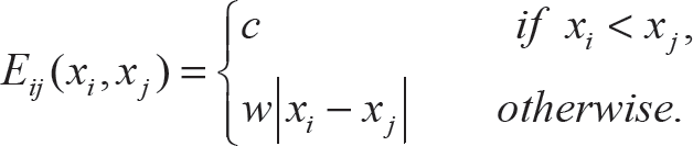
The smooth function E_ij(x_i, x_j) encodes the probability whereby neighbouring pixels should have a similar depth. Inspired by the work in [8], we use a linear cost function, which is solved by α-expansion:

E_{i j} (x_{i}, x_{j}) = w | x_{i} - x_{j} |

(6)

From the outdoor geometry, we know that objects which appear closer to the top of the image are usually further away. Thus, if we consider two pixels i and j, where j is directly above i, we have d_j > d_i according to the outdoor geometry. Thus, we can deduce that the transmission t_j of pixel j must be less than or equal to the transmission t_i of pixel i by using Eq. (2), that is x_j ≤ x_i. For any pair of labels which violate this trend, a cost c > 0 can be assigned to punish this pattern. Thus, the smoothing function in Eq. (6) can be written as:

E_{i j} (x_{i}, x_{j}) = {\begin{cases} c i f x_{i} < x_{j}, \\ w | x_{i} - x_{j} | o t h e r w i s e . \end{cases}

(7)

The parameters w and c are used to control the good or bad of the defogging effect. The value of w controls the strength of the detail enhancement, and is set usually between 0.01 and 0.1. The cost c controls the strength of the colour recovery, and is usually set between 100 and 1,000. The two parameters are useful as a compromise between highly enhanced details where colours may appear too dark, and less restored details where colours are brighter. Besides, the weights associated with the graph edge should be determined. If the intensities of two neighbouring pixels in the input foggy image I are less than 15 in each channel, which means that the two pixels have a high probability of sharing the same transmission value. Thus, the cost of the labelling is increased by fifteen-fold to minimize the artefacts due to the depth discontinuities in this case. Taking the data function and the smoothing function into the energy function equation (4), the pixel label of the transmission map can be estimated by using graph cut-based α-expansion. In our method, the gco-v3.0 library [17], developed by O. Veksler and A. Delong, is adopted for optimizing multi-label energies via the α-expansion. It supports energies with any combination of unary, pairwise and label-cost terms [18, 19]. Thus, we use the library to estimate each pixel label in an initial transmission map. The pseudo-code of the estimation process using the gco-v3.0 library is presented in Figure 5.

Figure 5.

The pseudo-code of the label assignment using the gco-v3.0 library

In Figure 5, M and N are the height and width of the input foggy image, and ω, w and c are the parameters in Eqs. (5) and (7). By using the functions defined in the optimization library (e-g., GCO_SetDataCost, GCO_SetSmoothCost and GCO_GetLabeling), we can obtain each pixel label x_t. Next, a proper intensity value of the initial transmission map can be assigned to each image pixel. Specifically, for each label x_i, we have:

t_{i n i} (x) = 255 - (x_{i} - 1) \times 8

(8)

In Figure 6, we show a synthetic example in which the image consists of five grey-level regions. The image can be accurately segmented into five label regions using the proposed MRF method, whereby the five labels are represented by five intensity values, whose results are shown in Figure 6.

Figure 6.

Synthetic example. (a) Input grey-level image. (b) Output multi-label image.

The MRF-based algorithm can also be applied to estimate the initial transmission map for real-world image. An illustrative example is shown in Figure 7. In the figure, Figure 7(b) shows the initial transmission map estimated using the algorithm presented above - its corresponding restored result is shown in Figure 7(c). One can clearly see that the appearance of the scene objects in the restored image looks one-dimensional.

Figure 7.

True example. (a) Input image. (b) Initial transmission map. (c) Restored result obtained using (b). (d) Bilateral filter to (b). (e) Restored result obtained using (d).

4.2.3 Refined transmission map estimation

As shown in Figure 7, there is an obvious deficiency in the recovered image in the discontinuities of the transmission map obtained by the MRF model. For example, the red bricks and the gaps between them should have the same depth values. However, as shown in Figure 7(b), one can clearly see the gaps between the bricks in the transmission map estimated by the MRF-based algorithm. In order to handle these discontinuities, many works adopt a bilateral filter to refine the transmission map estimation, such as local albedo-insensitive dehazing [20], filtering-based dehazing [21] and image dehazing using an iterative method [22], etc. In this work, we also apply a bilateral filter to our algorithm, since such a filter can smooth images while preserving edges [23]. Thus, the redundant details of the transmission map t_ini estimated by the algorithm presented above can be effectively removed, which improves the restored result with better detail enhancement capability. This process can be written as:

t (u) = \frac{\sum_{p ∊ N (u)} W_{c} (‖ p - u ‖) W_{s} (| t_{i n i} (u) - t_{i n i} (p) |) t_{i n i} (p)}{\sum_{p ∊ N (u)} W_{c} (‖ p - u ‖) W_{s} (| t_{i n i} (u) - t_{i n i} (p) |)}

(9)

where t_ini( u ) is the initial transmission map corresponding to the pixel u =(x, y) and N( u ) denotes the neighbours of u . The spatial domain similarity function W_c(x) is a Gaussian filter with the standard deviation σ_c: $W_{c} (x) = e^{- x^{2} / 2 σ_{c}^{2}}$ , and the intensity similarity function W_s(x) is a Gaussian filter with the standard deviation σ_s (it can be defined as: $W_{s} (x) = e^{- x^{2} / 2 σ_{s}^{2}}$ ). In our experiments, the values of σ_c and σ_s are set as 3 and 0.4, respectively. Thus, we can obtain the final refined transmission map, as shown in Figure 7(d–e), which is the restored result obtained using the refined map. From Figure 7(e), one can see that the restored result obtained using the bilateral filter has more layers and its stereoscopic depth perception seems more evident compared with the result (Figure 7(c)) obtained without using the filter. However, it takes about eight seconds to refine an initial transmission map of size 640×480 by executing MATLAB on a PC with a 3.00 GHz Intel Pentium Dual-Core Processor. In addition, although in our experiment we find that the filter can refine the map without creating significant errors in the restored image for our testing database, it may cause a gradient effect for some images due to the fixed parameter values σ_c and σ_s for different sizes of images.

4.3 Scene radiance recovery

Since, now, we already know the input haze image I(x), the final refined transmission map t(x) and the ambient light A, we can obtain the final fog removal image J(x) according to the image degradation model. The final defogging result J(x) is recovered by:

J (x) = \frac{I (x) - A}{\max (t (x), t_{0})} + A

(10)

where t₀ is application-based and is used to adjust the fog remaining at only the farthest reaches of the image. If the value of t₀ is too large, the result has only a slight defogging effect, and if the value is too small, the colour of the fog removal result seems oversaturated. Experiments show that when t₀ is set to 0.2, we can get visually pleasing results in most cases. An illustrative example is shown in Figure 8. In the figure, Figure 8(a) shows the input foggy images, Figure 8(b) shows the transmission map estimated by using our MRF-based method, and Figure 8(c) is the final defogging result.

Figure 8.

Image defogging example. (a) The input image. (b) Our transmission map. (c) The fog removal image.

5. Extension to Video and Application

5.1 Video defogging

Given the importance of the fog removal method, many researchers have studied algorithms for single image defogging. However, research into video defogging is rare in the literature. Video processing takes into consideration not only the pixel values in a single static frame but also the temporal relations between frames. For surveillance camera systems, the camera is fixed and often positioned high up, such that the background of each frame is unchangeable and the difference in the transmission map between a foreground object and the background is usually small. Thus, we can regard the foreground object as image noise and use some denoising algorithms - such as a bilateral filter - to eliminate the noise and produce a universal transmission map. Figure 9 shows the main idea behind our video processing method. During the defogging process, the transmission map is only calculated once for the background image of the input video and then applied to more frames with a tolerable error.

Figure 9.

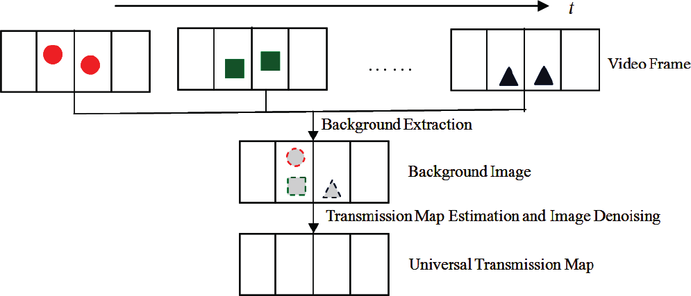
The main idea behind our video defogging process: Input video frames (top), extracted background image (middle) and estimated universal transmission map (bottom). In the input video frames, the foreground objects are denoted by circles, squares and triangles. These objects are regarded as image noise and are eliminated using a bilateral filter during the estimation process of the universal transmission map.

Specifically, we define the static part of the scene as the background part and the moving objects in the scene as the foreground part. The background image can be obtained by using a frame differential method. Next, our method estimates the transmission map of the background image by using the algorithm mentioned above as the universal transmission map, and applies the map to a series of video frames to obtain the restored images, as shown in Figure 10.

Figure 10.

Video results. First row: estimated background image and two original frames from the video. Second row: universal transmission map and the enhanced frames obtained by using the same transmission map.

The parameter values of the bilateral filter used in our video defogging method are set to a smaller value of σ_c and a larger value of σ_s (σ_c = 1, σ_s = 0.9) compared with single image defogging which cause the foreground noise and the redundant details of the transmission map to be effectively removed. Generally, no significant errors will be introduced into the restored image by using the universal transmission map, as shown in Figure 10.

5.2 Application

After acquiring the transmission map, we can add some visual effects on the fog removal image, such as fog simulation. Figure 11 shows the fog simulation results. The virtual foggy scene can be simulated by multiplying the extinction coefficient β by a factor of λ. Specifically, according to Eq. (2), this is achieved by applying the following simple power law transformation of the transmission values:

Figure 11.

Fog simulation based on our transmission map. (a) Input image. (b) and (c) Simulated foggy images with λ = 2 and λ = 4, respectively.

{(e^{- β d (x)})}^{λ} = t {(x)}^{λ}

(11)

where t(x) is the estimated transmission map. Once t(x) is computed, we can take the map into Eq. (10) to create the simulated fog scenes by adjusting parameter λ, as shown in Figure 11.

6. Experimental Results

6.1 Parameter setting

The proposed MRF model [see Eq. (7)] is mainly parameterized by w and c, which are the weights of the smooth term. From Figure 12, one can clearly see that the dents in the haystack are more obvious when w is close to 0.1 [see Figure 12(a)], and the colour of the fog removal results seems less saturated when c is close to 1,000 w [see Figure 12(b)].

Figure 12.

Defogging results with different parameter values. (a) From left to right: original image, the results obtained with w = 0.02 and c = 200w, w = 0.1 and c = 200w. (b) From left to right: original image, the results obtained with w = 0.05 and c = 200w, w = 0.05 and c = 1000w.

The value of w and c are application-based - we thus adopt the measurement presented in [24] to determine the proper value for the two parameters. For the CNC index proposed in that work, three components - contrast, image naturalness and colourfulness - are combined to yield an overall defogging result measure. Therefore, the CNC index between the original foggy image x and the fog removal image y is defined as:

C N C (x, y) = e {(x, y)}^{\frac{1}{5}} \cdot C N I (y) + C C I {(y)}^{\frac{1}{5}} \cdot C N I (y)

(12)

where e measures the contrast by the number of visible edges in image signals x and y, CNI is the image colour naturalness that describes the degree of correspondence between human perception and the external world, and CCI is the image colour colourfulness that presents the degree of colour vividness [25]. Good results are described by a high value of CNC. We use the CNC index as a feedback signal to determine the optimal value for the two parameters. Thanks to the feedback mechanism, the static, open-loop parameter estimation issue can be transformed into a dynamic parameter adjustment issue.

Figure 13 shows the average results of the CNC index with a different w and c for 128 testing images. One can clearly see that the best result, corresponding to the highest CNC value (1.2005), is obtained when w = 0.05 and c = 200w (see point M) for the testing images. Therefore, the optimal values for w and c are approximately 0.05 and 200w.

Figure 13.

Average results of CNC with different parameter values

We thus fix c = 200w and set an indicator of w over the range [0.1, 0.01] by a certain interval, which set as −0.001. The reason for us to choose CNC as a parameter adjustment index is that the index covers image contrast, naturalness and colourfulness. Besides, it is easy to implement and has quick computational speed. Assume that the index values obtained during a step are represented as CNC1 and CNC2, then the interaction conditions can thus be defined as: if CNC1 ≤ CNC2, iteration continues. Otherwise, stop the iteration and obtain the value of w in this condition. The defogging image produced with w and c (c = 200w) is our final result. Figure 14 shows the pseudo-code of the parameter estimation process.

Figure 14.

The pseudo-code of the parameter estimation using CNC

6.2 Synthetic Images

To evaluate the performance of various defogging algorithms, we rely on synthetic images due to the difficulty of acquiring a scene with and without fog. 66 synthetic images with uniform fog from the database FRIDA2 [26] are used here. This database contains ground-truth no-fog images as the target images to compare various defogging methods. The sample results obtained using the proposed MRF-based algorithm on the FRIDA2 databases are shown in Figure 15. One can see how far the extent to which the buildings and extends further in the restored images.

Figure 15.

Defogging results on synthetic images from the FRIDA2 database. First row: the synthetic images with fog. Second row: the obtained restored images using the proposed method.

We compared the proposed algorithm with the two classic enhancement algorithms: histogram equalization and the Retinex algorithm, as shown in Figure 16. Table 1 shows some of the results of the average absolute error (AAE) for the restored image and the target image without fog and for three defogging methods on 66 synthetic images with fog. In the evaluation, good results are described by a small value for the AAE. From Table 1, we can see that the proposed algorithm outperforms all the other algorithms. The AAE of the proposed algorithm is 30.71, while the next best result is 34.18 for the Retinex algorithm, which demonstrates that the results obtained with the proposed algorithm and the Retinex algorithm can effectively remove the fog. However, the remote object in our results seems much clearer than that seen using the Retinex method.

Figure 16.

Comparison of synthetic images. From left column to right column: original foggy image, results using histogram equalization, Retinex algorithm and the proposed algorithm.

Table 1.

Average absolute error between the restored image and the target image without fog

Algorithm	Mean error (in grey-levels)
Nothing	63.82
Histogram equalization	49.46
Retinex algorithm	34.18
Proposed method	30.71

6.3 Camera Images

The algorithms proposed in this paper work well for a wide variety of real captured foggy images. Figure 17 shows some examples of the defogging effects obtained using the proposed MRF-based algorithm. One can clearly see that the image contrast and detail are greatly improved compared with the original foggy images.

Figure 17.

Defogging results for real captured foggy images using the proposed method. First row: the real captured images with fog. Second row: the obtained restored images using the proposed method.

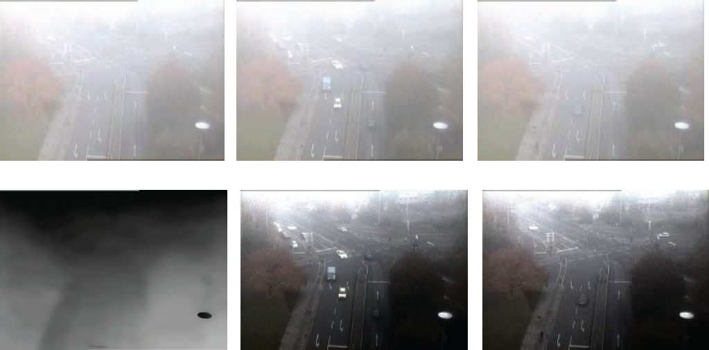
We also compared our defogging algorithm with several other state of the art algorithms. Figure 18 shows a comparison between the results obtained by Fattal [7] and our algorithm. As can be seen in Figure 18, Fattal's method can produce a visually pleasing result. However, the method is based on statistics and requires adequate colour information and variance. If the fog is dense, the colour information used in that method is not enough to reliably estimate the transmission.

Figure 18.

From left to right: the input image and the results obtained by Fattal [7] and our method

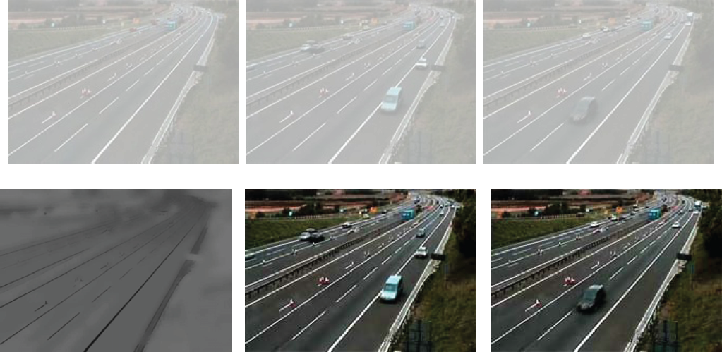
In addition, we compare our method with Tan's work [8] in Figure 19. The colours of Tan's result can sometimes over-saturate or distort. For example, the colour of the sky and the road region in Tan's result is turned yellow, as shown in Figure 19.

Figure 19.

From left to right: the input image and the results obtained by Tan [8] and our method

We also compare our method with He's work [2] in Figure 20. He's algorithm can achieve a good enhancement effect for most outdoor images. However, when the scene objects are inherently similar to the ambient light, the dark channel prior used in He's method will be invalid. In this case, the defogging result of He's algorithm is not visually pleasing, as shown in Figure 20.

Figure 20.

From left to right: the input image and the results obtained by He [2] and our method.

The comparison between the results obtained by Tarel [3] and our algorithm is shown in Figure 21. We can see that the colour in Tarel's result seems unnatural and that it also has many halo artefacts, whereas our method has no such problems.

Figure 21.

From left to right: the input image and the results obtained by Tarel [3] and our method.

Figure 22 shows a comparison between the results obtained by Carr [9] and our algorithm. It can be seen that our algorithm tends to enhance details better than Carr's result, and that the colour of our result seems closer to the original input image.

Figure 22.

From left to right: the input image and the results obtained by Carr [9] and our method

Figures 23 and 24 show the results of our method and Caraffa's methods [10, 11]. From these images, we can see that although the results we get are unable to thoroughly remove the fog in very dense fog regions compared with Caraffa's methods (e.g., the buildings and the trees in the distance), our results appear natural in terms of both colour and the profile of the scene objects.

Figure 23.

From left to right: the input image and the results obtained by Caraffa [10] and our method

Figure 24.

From left to right: the input image and the results obtained by Caraffa [11] and our method

Figure 25 shows a comparison between the results obtained by Wang [12] and our method. One can clearly see that the colour of the sky region in Wang's result seems a little inconsistent with that of the original foggy image.

Figure 25.

From left to right: the input image and the results obtained by Wang [12] and our method

Results on a variety of haze and fog images also show that the results obtained with our algorithm seem visually close to the results obtained by Carr, He and Fattal, with better colour fidelity and fewer halo artefacts than compared to Tan, Tarel, Caraffa and Wang. Meanwhile, we also find that - depending on the image - each algorithm is a trade-off between colour fidelity and contrast enhancement.

To quantitatively assess and rate the nine restoration algorithms (Fattal's method, Tan's method, He's method, Tarel's method, Carr's method, Caraffa's two methods, Wang's method and the proposed MRF-based method), we use the CNC index [24] to measure the defogging effect. Figure 18 to Figure 25 give some example results obtained using the above defogging algorithms, and their corresponding CNC results are shown in Table 2. From the table, we can see that the highest values of CNC are obtained using the proposed method. This illustrates that the proposed method can achieve as good or even better results in most real-world foggy situations as compared to other defogging algorithms.

Table 2.

CNC index computed for the nine compared methods

Figure	Image defogging methods
	[7]	[8]	[2]	[3]	[9]	[10]	[11]	[12]	Our
18	1.83	1.69	1.97	1.77	1.20				2.07
19	1.26	1.24	1.16	1.19	1.24				1.36
20	2.01	1.96	2.16	0.99	2.19				2.29
21	1.11	1.09	1.09	0.95	1.11				1.13
22	1.28	1.19	1.23	0.94	1.27				1.43
23	1.18	1.08	1.10	0.79	1.21	1.16			1.24
24	1.79	1.69	1.73	1.76	1.80		1.74		1.82
25	1.96	1.87	1.91	1.87	2.02			1.88	2.04

To better evaluate the proposed method, an assessment method dedicated to visibility restoration proposed in [27] is also used here to measure the contrast enhancement of the defogged images. We first transform the colour-level image to a grey-level image and use the three indicators to compare two grey-level images: the input image and the fog removal image. The visible edges in the image before and after restoration are selected by a 5% contrast threshold according to the meteorological visibility distance proposed by the International Commission of Illumination. To implement this definition of contrast between two adjacent regions, the method for the segmentation of visible edges proposed in [28] has been used.

Once the map of the visible edges is obtained, we can compute the rate e of edges that are newly visible after restoration. Next, the mean $\bar{r}$ over these edges of the ratio of the gradient norms both before and after restoration is computed. This indicator $\bar{r}$ estimates the average visibility enhancement obtained by the restoration algorithm. Finally, the percentage of pixels σ which become completely black or completely white after restoration is computed.

These indicators e, $\bar{r}$ and σ are evaluated for Fattal [7], Tan [8], He [2], Tarel [3], Carr [9], Caraffa [10, 11], Wang [12] and our method on eight images (see Table 3).

Table 3.

Comparison of the state of art defogging algorithms with the three indicators

Indicator	e	$\bar{r}$	σ	e	$\bar{r}$	σ
Method	Figure 18 (512×384)			Figure 19 (600×400)
Fattal^[7]	0.319	2.399	0.008	0.416	1.149	0.490
Tan^[8]	0.346	3.418	0.274	0.536	3.123	0.849
He^[2]	0.312	1.266	0.023	0.676	1.607	0.074
Tarel^[3]	0.351	2.169	0	0.532	2.016	0
Carr^[9]	0.218	2.785	0.005	0.022	2.462	0.006
Caraffa^[10]
Caraffa^[11]
Wang^[12]
Our	0.151	3.709	0.052	0.604	2.176	0.365
Method	Figure 20 (400×300)			Figure 21 (640×480)
Fattal^[7]	3.264	1.592	0.688	1.592	2.297	0.402
Tan^[8]	4.537	2.594	0.983	2.185	2.897	0.571
He^[2]	3.975	1.720	0.052	1.814	2.361	0.240
Tare^[3]	0.936	2.259	0	0.820	2.250	0
Carr^[9]	0.842	1.653	0.003	1.494	2.017	0.001
Caraffa^[10]
Caraffa^[11]
Wang^[12]
Our	3.619	1.677	0.882	0.715	1.740	0.349
Method	Figure 22 (480×270)			Figure 23 (493×329)
Fattal^[7]	2.895	1.508	0.377	1.224	1.392	0.798
Tan^[8]	4.217	3.062	0.492	1.854	2.754	0.983
He^[2]	3.122	1.640	0.274	1.252	1.431	0.851
Tarel^[3]	2.546	2.614	0	1.036	2.305	0
Carr^[9]]	1.371	1.617	0	1.004	1.937	0.002
Caraffa^[10]				1.080	2.420	0.001
Caraffa^[11]
Wang^[12]
Our	2.603	2.297	0.168	1.144	1.953	0.080
Method	Figure 24 (505×364)			Figure 25 (700×520)
Fattal^[7]	0.182	1.963	0.464	0.499	0.673	0.104
Tan^[8]	0.686	2.971	0.637	1.679	2.483	0.286
He^[2]	0.196	0.948	0.132	0.596	0.837	0.059
Tarel^[3]	0.524	2.635	0.001	1.106	2.255	0.001
Carr^[9]	0.407	1.379	0	0.887	1.379	0.007
Caraffa^[10]
Caraffa^[11]	0.253	1.787	0.210
Wang^[12]				0.542	1.364	0.033
Our	0.425	1.393	0.034	0.921	1.445	0.134

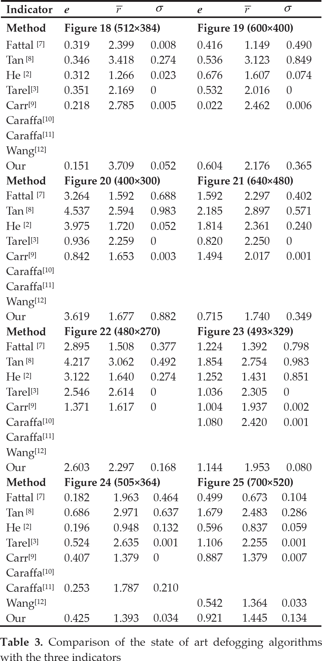
Under each method, the aim is to increase the level of contrast without losing visual information. Hence, according to [27], good results are described by high values of e and $\bar{r}$ and low values of σ. From Table 3, we deduce that, depending on the image, Tan's algorithm generally has more visible edges than the other algorithms. Moreover, we can order the algorithms in decreasing order with respect to the average increase in the degree of contrast on the visible edges: Tan, Tarel, He, Fattal, Caraffa, our own, Carr and Wang. However, in the experiment we find that the algorithms with more visible edges probably increase the contrast to much, such that the defogged images may have halos near some edges and the colour following defogging seems unnatural. This confirms our observations regarding Figure 18 to Figure 25.

6.4 Video defogging results

Experimental results with videos of traffic scenes taken under foggy conditions are offered in Figures 26 and 27. The two video clips are used to evaluate the proposed algorithm for traffic monitoring. One clip has 350 frames, with 768×576 RGB colour images coded with 24 bits per pixel. The other is a 640×480 resolution 200-frame video. As described in previous experiments, we first obtain the background image of the input foggy video sequences and compute the universal transmission map for the background image. Next, the contrasts of the road, trees and moving vehicles were restored for each frame of the video using the universal map. Notice the significant increase in contrast and the improvement in colour (see Figures 26 and 27). In our current implementation, fog removal was applied to the input foggy video while offline.

Figure 26.

Restoration results for video clip #1. First row: estimated background image and two original frames from the video. Second row: universal transmission map and the enhanced frames obtained using the universal map.

Figure 27.

Restoration results for video clip #2. First row: estimated background image and two original frames from the video. Second row: universal transmission map and the enhanced frames obtained using the universal map.

6.5 Computation times

The computational time is measured by executing MATTAB on a PC with a 3.00 GHz Intel Pentium Dual-Core Processor.

For an image of size s_x×s_y, the fastest algorithm is Tarel's method. The complexity of Tarel's algorithm is O(s_xs_y), which implies that the complexity is a linear function of the number of input image pixels. Thus, only two seconds are needed to process an image of size 600×400. For He's method, its time-temporal complexity is relatively high, since the Matting Laplacian matrix L used for the method is so large; therefore, for an image of size s_x×s_y, the size of L is s_xs_y×s_xs_y; accordingly, 20 seconds are needed to process a 600×400 pixel image. The computational times of Fattal's and Tan's methods are even greater than that of He's method. They take about 40 seconds and five to seven minutes to process a foggy image of the same size, respectively. For our proposed algorithm, it takes about two minutes to process a 600×400 pixel image. This can be improved using a GPU-based parallel algorithm. Notice that when the image size is small, the proposed method has a relatively faster speed. For example, only three seconds are needed to process a 250×190 pixel image using our method, while it takes about six seconds to process an image of the same size using He's method.

7. Conclusions

Image defogging is an important issue in computer vision. In this paper, a new defogging algorithm was presented based on a MRF model. The problem was formulated as the estimation of a transmission map with α-expansion optimization. The algorithm was implemented in two stages. First, the transmission map was estimated using a dedicated MRF model and a bilateral filter. Second, once the map was inferred, the restored image could be obtained according to the image degradation model.

The experimental results demonstrated that the proposed algorithm can produce visually pleasing defogging results and that it tends to enhance the image contrast, which is better than previous techniques. The main contributions of this work are as follows:

(1)

A novel MRF-based method was proposed which applies an optimization library to estimate a transmission map. Experiments on both synthetic images and real-world images showed the effectiveness of the proposed method.

(2)

We extended our proposed method to foggy video applications using the universal strategy and implemented the fog environment simulation based on the estimated transmission map.

(3)

Due to the feedback mechanism proposed in this paper, the static open-loop parameter estimation issue can be transformed into a dynamic parameter adjustment issue.

However, the colour of our defogging results sometimes seemed over-saturated, and some fog removal results may have a gradient effect. Nevertheless, we might improve the overall quality of a foggy image by enhancing the main details, and the algorithm could be further improved by employing better image prior for the smoothing function of the MRF model. In the future, we intend to investigate instances of various kinds of fog and speed up the proposed algorithm for real-time processing.

Footnotes

8.

The authors would like to thank Dr. Fan for providing his paper [], Dr. Tarel for providing the MATLAB code for his approach, and Dr. Fattal, Dr. Tan, Dr. He and Dr. Carr for providing the defogging images on their websites. This work was supported by the National Natural Science Foundation of China (71271215, 71221061 and 91220301), the International Science and Technology Cooperation Programme of China (2011DFA10440), the Collaborative Innovation Centre of resource economical and environment friendly society, the China Postdoctoral Science Foundation (No. 2014M552154), the Hunan Postdoctoral Scientific Program (No. 2014RS4026), and the Postdoctoral Science Foundation of Central South University (No. 126648).

References

[1] Yu

B N

Kim

B S

Lee

K H

, (2012) Visibility enhancement based real-time Retinex for diverse environments. The 8th International Conference on Signal Image Technology and Internet Based Systems (SITIS), Sorrento, Naples, Italy. USA: IEEE. 72–79.

[2] He

K M

Sun

Tang

X O

, (2011) Single image haze removal using dark channel prior. IEEE Transactions on Pattern Analysis and Machine Intelligence. 33(12): 2341–2353.

[3] Tarel

J P

Hautiere

, (2009) Fast visibility restoration from a single color or gray level image. IEEE International Conference on Computer Vision (ICCV), Kyoto, Japan. USA: IEEE. 2201–2208.

[4] Li

S Z

, (2009) Markov random field modeling in image analysis. UK: Springer-Verlag London Limited. 21.

[5] Nishino

Kratz

Lmbardi

, (2012) Bayesian defogging. International Journal of Computer Vision. 98(3): 263–278.

[6] Kratz

Nishino

, (2009) Factorizing scene albedo and depth from a single foggy image. IEEE International Conference on Computer Vision (ICCV), Kyoto, Japan. USA: IEEE. 1701–1708.

[7] Fattal

, (2008) Single image dehazing. ACM Transactions on Graphics. 27(3): 1–9.

[8] Tan

R T

, (2008) Visibility in bad weather from a single image. IEEE international conference on computer vision and pattern recognition (CVPR), Anchorage, Alaska, USA. USA: IEEE. 1–8.

[9] Carr

Hartley

, (2009) Improved single image dehazing using geometry. The Digital Image Computing: Technique and Applications, Melbourne. USA: IEEE. 103–110.

10.

[10] Cataffa

Tarel

J P

, (2013) Markov random field model for single image defogging. IEEE Intelligent Vehicle Symposium, Gold Coast. USA: IEEE. 994–999.

11.

[11] Caraffa

Tarel

J P

, (2012) Stereo reconstruction and contrast restoration in daytime fog. Asian Conference on Computer Vision (ACCV), Daejeon, Korea. UK: Springer. 13–25.

12.

[12] Wang

Y K

Fan

C T

Chang

C W

, (2012) Accurate depth estimation for image defogging using Markov Random Field. International Conference on Graphic and Image Processing (ICGIP), Singapore. USA: SPIE Digital Library. 1–5.

13.

[13] Kolmogorov

Zabin

, (2004) What energy function can be minimized via graph cuts? IEEE Transactions on Pattern Analysis and Machine Intelligence (PAMI), 26(2): 147–159.

14.

[14] Boykoc

Kolmogorov

, (2004) An experimental comparison of min-cut/max-flow algorithms for energy minimization in vision. IEEE Transactions on Pattern Analysis and Machine Intelligence (PAMI), 26(9): 1124–1137.

15.

[15] Rossum

M V

Nieuwenhuizen

, (1999) Multiple scattering of classical waves: microscopy, mesoscopy and diffusion. Reviews of Modern Physics, 71(1): 313–371.

16.

[16] Narasimhan

S G

Nayar

S K

, (2002) Vision and the atmosphere. International Journal on Computer Vision, 48(3): 233–254.

17.

[17] The gco-v3.0 library (gco-v3.0). Available: http://vision.csd.uwo.ca/code/ Accessed on 5 April 2013.

18.

[18] Boykov

Veksler

Zabin

, (2001) Fast approximate energy minimization via graph cuts. IEEE Transaction on Pattern Analysis and Machine Intelligence (PAMI), 23(11): 1222–1239.

19.

[19] Delong

Osokin

Isack

H N

Boykov

, (2012) Fast Approximate Energy Minimization with Label Costs. International Journal of Computer Vision, 96(1): 1–27.

20.

[20] Zhang

J W

Yang

G Q

Zhang

, (2010) Local albedo-insensitive single image dehazing. Visual Computer, 26:761–768.

21.

[21] Xiao

C X

Gan

J J

, (2012) Fast image dehazing using guided joint bilateral filter. Visual Computer, 28:713–721.

22.

[22] Sun

Wang

Zheng

Z H

Zhou

Z Q

, (2010) Fast Single Image Dehazing Using Iterative Bilateral Filter. International Conference on Information Engineering and Computer Science (ICIECS), Wuhan, China: IEEE. 1–4.

23.

[23] Tomasi

Manduchi

, (1998) Bilateral Filtering for Gray and Color Images. IEEE International Conference on Computer Vision (ICCV), Mumbai, India. USA: IEEE. 839–846.

24.

[24] Guo

Tang

Cai

Z X

, (2014) Objective measurement for image defogging algorithms. J. Cent. South Univ. 21(1): 272–286.

25.

[25] Huang

K Q

Wang

Z Y

, (2006) Natural color image enhancement and evaluation algorithm based on human visual system. Computer Vision and Image Understanding. 103(1): 52–63.

26.

[26] Tarel

J P

Hautiere

Caraffa

Cord

Halmaoui

Gruyer

, (2012) Vision enhancement in homogeneous and heterogeneous fog. IEEE Intelligent Transportation Systems Magazine, 4(2): 6–20.

27.

[27] Hautiere

Tarel

J P

Aubert

Dumont

, (2008) Blind contrast enhancement assessment by gradient ratioing at visible edges. Image Analysis & Stereology Journal, 27(2): 87–95.

28.

[28] Kohler

, (1981) A segmentation system based on thresholding. Graph Model Im Proc, 15(3): 319–338

A Markov Random Field Model for the Restoration of Foggy Images

Abstract

Keywords

1. Introduction

2. Previous Works

3. Background

3.1 Markov Random Fields

4.1 The algorithm flowchart

4.2.2 Initial transmission map estimation

5.1 Video defogging

6.1 Parameter setting

7. Conclusions

Footnotes

8.

References