
Abstract
Wire-moving robots are mechanical systems that can maintain their balance and move on tightropes. Their name comes from the manner in which tightrope walkers maintain their balance by rolling or moving a pole from left to right. In order to investigate the internal laws of these systems and to apply a mechanism of self-balance control to them, a new mechanical structure for wire-moving robots is presented here. This structure consists of a rotational pole and a translational pole coupled with each other in a parallelogram. The robot is an underactuated system. A dynamic model of the robot is established here based on the Lagrange method, and the controller of the system was designed using a partial feedback linearization control algorithm. Finally, the efficiency of the algorithm and the stabilization were verified by computer simulation and experimentation using a prototype.
1. Introduction
High-wire acts have a long history. Even for a skilled acrobat it is difficult to maintain balance on a wire using only a long pole, and it is also dangerous. Many researchers have tried to realize this kind of self-balance control using mechanical devices. In 2005, a mobile robot suspended on wire was designed by Rogério Sales G and João Carlos Mendes C [1], as shown in Figure 1. The robot has four legs that move like a human climbing beneath a single wire.

A four-legged wire-moving robot
A two-wheeled wire-moving robot was also designed based on the gyroscopic effect [2]. In one study, a robot suspended on overhead ground wires was designed with a controller capable of obstacle-navigation control [3]. Its localization method and database were based on two laser sensors. Almost all wire-moving robots are designed so that most of the robot's mass is beneath the wire. Producing a wire-moving robot whose bulk remains above the wire is a new challenge.
Many wire-moving robots have been designed for the inspection of power transmission lines [3–9] and this kind of robot is used widely. The Expliner and LineScout robots are two examples.
The Expliner robot was designed by the Kansai Electric Power Company HiBot, and the Tokyo Institute of Technology. It is an inspection robot used on ultra-high voltage power lines [8]. The main part of the Expliner robot is located below the power lines and hangs below two parallel wires by eight wheels, four on each wire, as shown in Figure 2. The Expliner robot can inspect the wires and repair failed or damaged areas. The Expliner robot can even cross some of the barriers on the wires.

The Expliner robot
The LineScout robot was designed by the Hydro Québec Research Institute. It is the best inspection robot for ultra-high voltage power lines currently available [9], as shown in Figure 3. Like the Expliner robot, the bulk of the LineScout robot is also below the wires. However, the LineScout robot can hang below only one wire. This allows the LineScout robot to cross most kinds of fittings on the wires. Its mechanical arm can perform complex actions, like replacing vibration dampers on the wires.
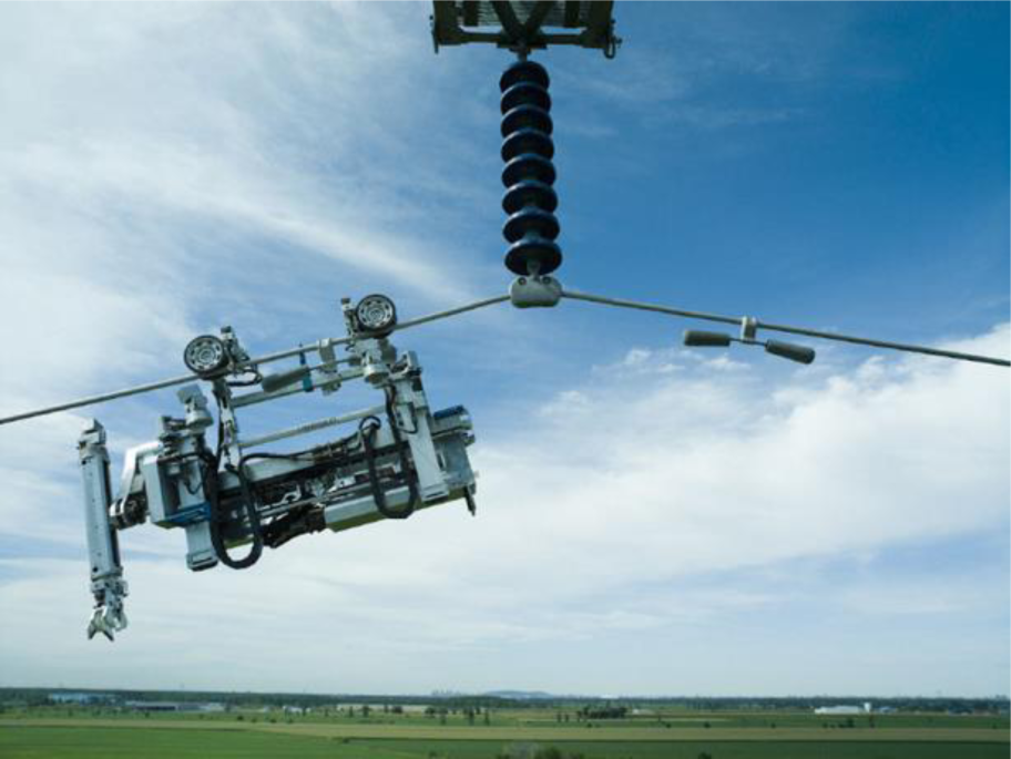
The LineScout robot
The difference between the wire-moving robot in this paper and the two robots (Expliner and LineScout) above is that all parts of our wire-moving robot are located above the wire. The robot moves on only one wire and maintains its balance by rotating the rotational pole and moving the translational pole. This wire-moving robot was modelled on the movements of a tightrope walker. This robot can be used to explore the theory underlying the mechanisms by which robots maintain their balance while travelling on one wire. Studies of this kind can be used to design tightrope-moving robots for entertainment and for applications in which a robot must be able to manoeuvre on top of a wire instead of beneath it.
Overall, although all the robots can move steadily across thick wires, they differ from each other considerably. Most types of these robots maintain their balance more easily because their centres of mass are below the wire.
One previous study presents the dynamic model and controller design of a wire-moving robot capable of maintaining its balance through control of a rotational pole [10]. A computer simulation was used to verify the results of the theoretical analysis. These were the early results of our research. However, the paper does not discuss the effect of the translational pole for the robot self-balancing control. Neither does it describe the production of a real prototype or experimental environment. This is the primary consideration of the present work.
The structure and design of a new wire-moving robot are described in this article. The robot was controlled using both a rotational pole and a translational pole. These poles were coupled using a parallelogram structure, which was intended to simulate the control exerted by a human arm when driving the balancing pole. To distinguish between these two kinds of robot, the robot with two poles is here called the rotational and translational pole (RTP) robot and the other is called the rotational pole (RP) robot. The RP robot was first presented in a previous study [10].
The dynamic model of the system was established using the Lagrange method [11], and the controller was designed using the partial feedback linearization control algorithm [12]. The validity and the stabilization were confirmed by the computer simulation and by experiments based on the real prototype.
2. Mechanical design
The purpose of the wire-moving robot was to investigate the internal laws by which humans maintain their balance while walking on a high-wire and to apply this type of self-balance control to a mechanical system. In this section, the mechanical structure of the wire-moving robot is described.
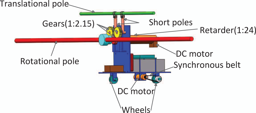
The wire-moving robot is a mechanical system that can maintain its balance and move on tightropes. The wire-moving robot was designed using some of the same theories that underlie the motion of acrobats as they maintain their balance on a tightrope. In a high-wire performance, the acrobat holds a long pole. When the acrobat's centre of mass (COM) moves, the acrobat rotates the long pole in the direction of the COM. The COM is affected by the counter-torque of rotating the pole. The acrobat then inclines his or her body in the direction opposite to the rotation of the pole. This causes the COM to return to the equilibrium position. The mechanical structure of the wire-moving robot is shown in Figure 4. The rotational pole in the front portion of the robot serves the same function as the long pole in the acrobat's hand, and the motor fixed to the rotational pole acts as the acrobat's wrist. The translational pole, which is behind the rotational pole, serves as the acrobat's body. When the COM of the robot moves, the robot rotates the rotational pole in the direction of the COM to shift it. At the same time, the small gear that is fixed with the rotational pole rotates with the rotational pole and turns the two large gears that are fixed to the hinges on the translational pole. In this way, the translational pole moves horizontally to the opposite side of the rotational pole and the COM returns to the equilibrium position. Because acrobats only need to incline their bodies by a small angle to move their COMs back to the equilibrium position, the gear fixed to the rotational pole is smaller than the gears fixed to the short poles that control the angle of the translational pole. There are two wheels set along a single line on the robot's chassis. The wheel under the robot serves as the acrobat's feet and is used to move the robot forward.

Conceptual design of the RTP robot
The translational pole is fixed to the two bushings. The two bushings are connected to the two parallel short poles by two hinges, one per pole. The two short poles are fixed to the two large gears, one to each. When the small gear turns, the two large gears are also turned by the small gear and the two short poles. Then the translational pole moves horizontally. In this way, a parallelogram structure is formed by the translational pole and the two short poles.
A simple depiction of the parallelogram structure is given in Figure 5. If link AD and link BC rotate in the same direction, the centre of mass of link CD will move away from the original position and reach a new equilibrium position.

Parallelogram structure
Incorporating both observations of human tightrope walkers and studies of mechanical structures, the wire-moving robot was designed as a two-wheeled mechanical system, as shown in Figure 6.
Assembly of the RTP robot
One of the two wheels under the robot is driven by a small DC motor to make the robot move forward. The rotational pole is also driven by a DC motor. The translational pole can move horizontally when the large DC motor rotates the rotational pole.
3. Dynamic model
In this section, the dynamic model of the wire-moving robot, as shown in Figure 7, is described. It was developed using the Lagrange method.

Wire-moving RTP robot with the definition of the coordinate systems
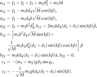
Here, p1 represents the integrated COM of the robot's body and the rotational pole, p2 represents the COM of the rotational pole and p3 represents the COM of the translational pole.
The reference coordinate system oxyz is established with the origin at one end of the rope, axis x passing through the rope, and axis z perpendicular to the ground. The local coordinate system o1y1x1z1 is attached to the robot's body with the origin o1 located at the point where the rope crosses the line passing through p1 and is perpendicular to the ground. Axis x passes through the rope and axis z is parallel to the plumb line. The local coordinate system o2x2y2y2c2 is attached to the rotational pole with the origin o2 located at p2. The local coordinate system o3x3y3z3 is attached to the translational pole with its origin o3 located at p3. α is the relative angle between the coordinate systems o1y1x1x1z1 and oxyz, and β is the relative angle between the coordinate systems and o1y1x1z1. α and β denote the corresponding angle velocity values.
In order to build the dynamic model based on the Lagrange theorem, it was assumed that the rope was tight so as to never swing while people were walking on it.
J1 served as the moment of inertia of the robot body around axis o1x1. J2 was the moment of inertia of the rotational pole around axis o2x2, J3 was the moment of inertia of the translational pole. l2 was the length of the rotational pole, d1 was the distance from point c to the rope. d2 was the distance from point c2 to the rope. l3 was the length of the translational pole. d3 was the distance from the rotation centre A or B of the parallelogram structure to the rotational pole. d4 was the length of the connecting link of the parallelogram structure. d5 was the distance between the translational pole and the rope, m1 was the mass of the robot body, m2 was the mass of the rotational pole, m3 was the mass of the translational pole, and g was the acceleration of gravity.
The robot moves around the rope with the angular velocity α̇, so the rotational pole does as well. At the same time, the rotational pole is driven by a motor with the angular velocity β̇. Therefore its total angular velocity is d2α̇ and its translational velocity is α̇ + β̇. The angular velocity of the translational pole is α̇ and its translational velocity is d5α̇, where d5 = √M and the following is true:

As shown in Figure 8, as the rotational pole moved with the angular velocity of β̇, the angle θ of the connecting link of the parallelogram turned as follows:


Analysis of the parallelogram structure
4. Design of the controller
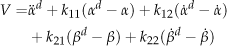
According to the first equation of (13), the new equation of α̈ is expressed as follows:
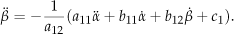


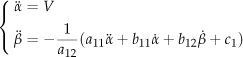
The controller was designed as follows:

The structure of the controller is shown in Figure 9.
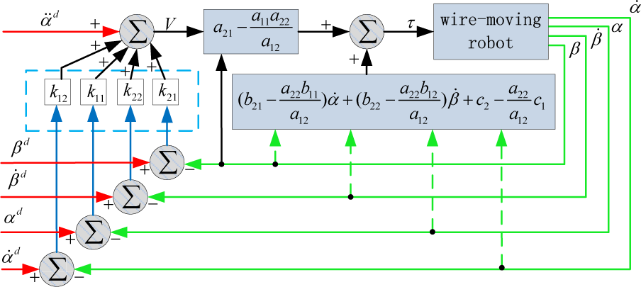
Structure of the controller
5. Stability of the system
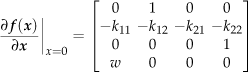
At the equilibrium point of the system, the Jacobian matrix of (20) is as follows:


6. Computer simulation
6.1 Establishment of the virtual prototype
The virtual prototype is designed in SolidWorks, and the SolidWorks model was imported into Adams and analysed. As shown in Figure 10, all of the robot parts were constrained by each other. Based on the assumption given above, the wire was designed to act as a rigid body, and it was fixed to the ground.

Virtual prototype of the RTP robot
The parameters of the virtual prototype are given in the following table.
6.2 Process and results of the simulation of the motion of the RTP robot
Virtual prototype parameters of the RTP robot


Roll angle and relative rotation of the rotational pole of the RTP robot
Motor control torque of the RTP robot
In Figure 11, the red solid line represents the roll angle of the robot. The blue dotted line represents the relative rotation of the rotational pole. All the peaks in the solid line are opposite to those on the dotted line. As the rotational speed of the rotational pole increased, the roll angle of the RTP robot decreased. Three seconds later, the robot had almost reached equilibrium. At the same time, the rotational pole and the translational pole continued to move at low speed. This had little influence on the roll angle of the robot body. Four seconds later, the roll angle of the robot body had decreased from the initial angle of 10° to 0°, and the relative angle between the rotational pole and the robot body had decreased from the maximum angle of 80° to 0°. The RTP robot system became stable.
In Figure 12, the red solid line represents the control torque of the DC motor. This curve has the same shape as the roll angle in Figure 11. This means that the motor rotates in the same direction as the movement of the RTP robot. It takes only four seconds for the curve to converge during the control process. This shows that the controller is highly effective. Human performers perform similar actions to maintain their balance while walking on a wire. In conclusion, the simulation result demonstrated the internal law of tightrope walking.
6.3 Comparison of the RTP and RP robots
The establishment of the controller design and the simulation model of the RP robot can be seen in a previous study [10]. The simulation of the RP robot presented in a previous study is here compared to the simulation of the RTP robot[10].
Figure 5 of the previous study is here compared to Figure 11. The settling time of the response of RP robot's roll angle was about 3s. However the RTP robot took only about 1.5s. The two curves of the responses of the roll angle show that the RTP robot has a considerable advantage over the RP robot with respect to overshoot. Figure 6 of the previous study is compared to Figure 12 of the current study. The motor torque curve of the RTP robot also showed a shorter settling time and less overshoot. In this way, the response of the RTP robot was found to converge faster and show less vibration frequency than the response of the RP robot under the same initial conditions. Overall, the performance index of the control system had increased significantly after the addition of the translational pole to the robot.
7. The experiments
7.1 Physical prototype
The physical prototypes of the RTP and RP robot are shown in Figure 13. The TMS320F28335 DSP controller serves as the core processor of the control systems. The whole system is shown in the block diagram as shown in Figures 14 and 15.

RTP and RP wire-moving robot 1- Rotational pole. 2- MTi gyroscope. 3- Battery. 4- DSP controller. 5- Photo electricity encoder. 6- Gesture adjustment DC motor. 7- Translational pole. 8- Gears
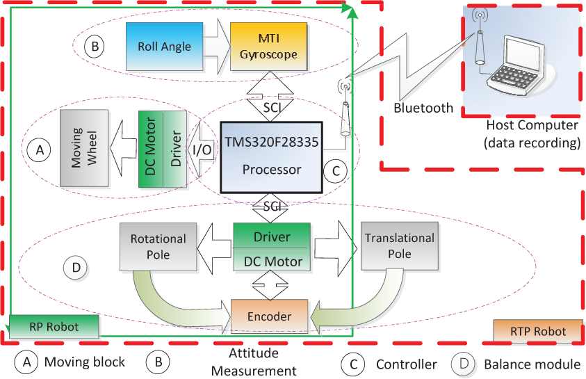
Block diagram of the system

Physical devices of the system
Figure 15 shows the physical devices of the system and how they are connected to each other.
7.2 Rigid rail experiments
The parameters of the physical prototype were recalculated, producing the values of the mechanical system. They are shown in Table 2. The experiment was carried out on a guide rail.
The physical parameters of the robots

7.2.1. RTP robot on a rigid rail
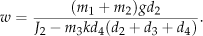
According to Table 2, the constant w which is described in Eq. (22) can be calculated as 25.2238. The four parameters were adjusted as follows.

Then the roots of equation 22 were recalculated as follows. The system was found to be asymptotically stable.
The results are shown in Figures 16 and 17.
RTP robot on the rigid rail
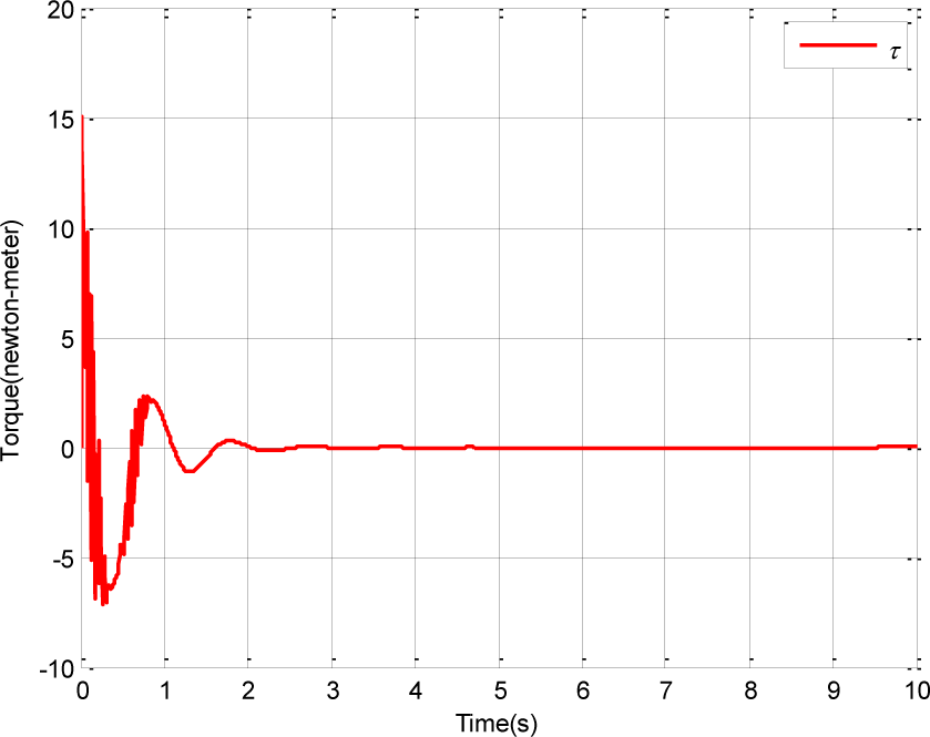
DC control torque of the RTP robot
The robot was set to its equilibrium position at the beginning. Then a horizontal interference force was exerted upon the robot between the third and fourth seconds. Then the roll angle increased to 10°. The controller quickly took effect, and the system began to converge. Two seconds later, the roll angle decreased to 0°. Finally, the robot oscillated near equilibrium within a range of ±3°, as in the simulation. This showed the control algorithm to be effective. By observing Figure 17, the curve of the torque was found to be similar to the roll angle in Figure 16 and it was concluded that the system is dynamically stable.
The following experiment, shown in Figure 18, was performed to assess the stability of the robot in situations involving dynamic interference. Interference was exerted upon the robot three times in different directions over the course of 18s. The robot remained stable every time and never fell off of the guide rail.
The roll angle of the RTP robot under interference
7.2.2. RP robot on a rigid rail
The physical prototype was designed for a simulation and is shown in Figure 13(b). The core processor of the robot's measurement and control system is DSP28335. The system can be used to determine the control torque using data obtained from a sensor system which are sent to the motor drive. Then the motor would rotate the rotational pole to maintain its balance.
As in Table 2, the four parameters were adjusted using the robot's data. This produced the following four parameters:


The experiment results are shown in Figures 19 and 20.

The roll angle of the RTP robot under interference

Motor output torque of the RP robot on the rigid rail
As shown in Figure 19, a horizontal interference force was exerted upon the robot at the equilibrium position. This caused a depression in the red curve. At the same time, the rotational pole rotated toward the direction in which the robot had inclined, causing the robot to return to the equilibrium position. Then overshoot increased the roll angle of the robot to nearly 10°. The controller quickly rotated the rotational pole to nearly 55°, moving the COM of the robot to the equilibrium position. In the end, the robot reached the dynamic stable state near the equilibrium position. Motor output torque over time is shown in Figure 20.
The robustness of the robot is shown in Figure 21. Interference was imposed upon the system 2s into the experiment. The roll angle of the robot converged to less than 2°4s into the experiment. Interference was reimposed at 8s and the robot again returned to the equilibrium position quickly. Then the amplitude of the third disturbance was increased, which increased the roll angle of the robot to 8°. The controller worked effectively and the robot regained its balance after 3s. After several rounds of interference of different amplitudes, the robot maintained its balance and did not fall off the rigid pole. This showed the controller to be able to foster stability.

Roll angle of the RP robot on the rigid rail with disturbance
7.2.3. Comparison of RTP and RP robots on a rigid rail
The actual experimental results are shown in Figures 16 and 19. They indicate that the roll angle of the RP robot ranged from about −3 ~ 23°. The stability of the RP robot was about −3 ~ 3°. However, the roll angle of the RTP robot was about −3 ~ 9°, and the stability of the RTP robot was about −3 ~ 3°. The largest angle of the rotational pole of the RP robot was nearly 50°. However, the largest angle of the rotational pole of the RTP robot was only 35°. This shows that the RTP robot can be balanced by controlling the rotational pole with a relatively small angle. Figures 18 and 21 show that the range of the output torque of the RTP robot is smaller than the range of RP robot when both are subject to interference.
An attempt was made to test the RP robot on a flexible wire, but the robot showed a negligible ability to maintain its balance. The RP robot was rebuilt as an RTP robot for the flexible wire experiments.
7.3 RTP robot on a flexible wire
The rigid rail was replaced with a flexible wire. The experimental platform is shown in Figure 22.

Flexible wire experiment platform
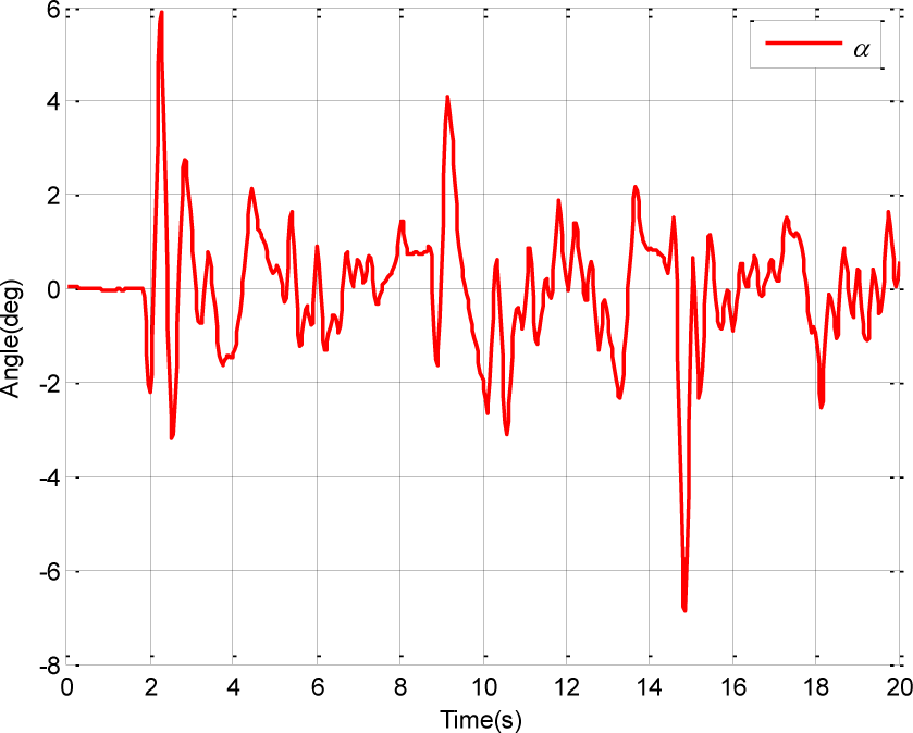
Because the wire is flexible, the RTP robot cannot be set at the equilibrium position statically. It can only be set at a position near its equilibrium. An experiment without any interference is shown in Figure 23. The RTP robot was found to remain dynamically stable on the wire and its roll angle was very small, varying within a range of ±3°.

RTP robot on the wire
As shown in Figure 24, the control torque varied within the range of ±5Nm, excepting one large fluctuation at 14s. However, the controller then took effect quickly and the RTP robot returned to the equilibrium position. In this way, the RTP robot was found to perform well on the wire when no interference was deliberately added. Another experiment was performed in order to assess the performance of the RTP robot under conditions involving human interference. It is shown in Figures 25 and 26.

Control torque of the motor for the RTP robot on the wire
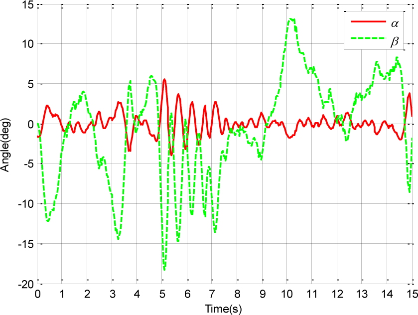
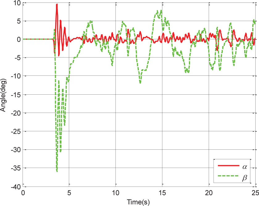
RTP robot on the wire with interference
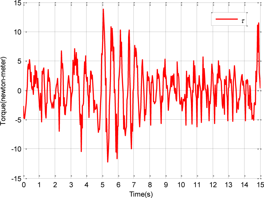
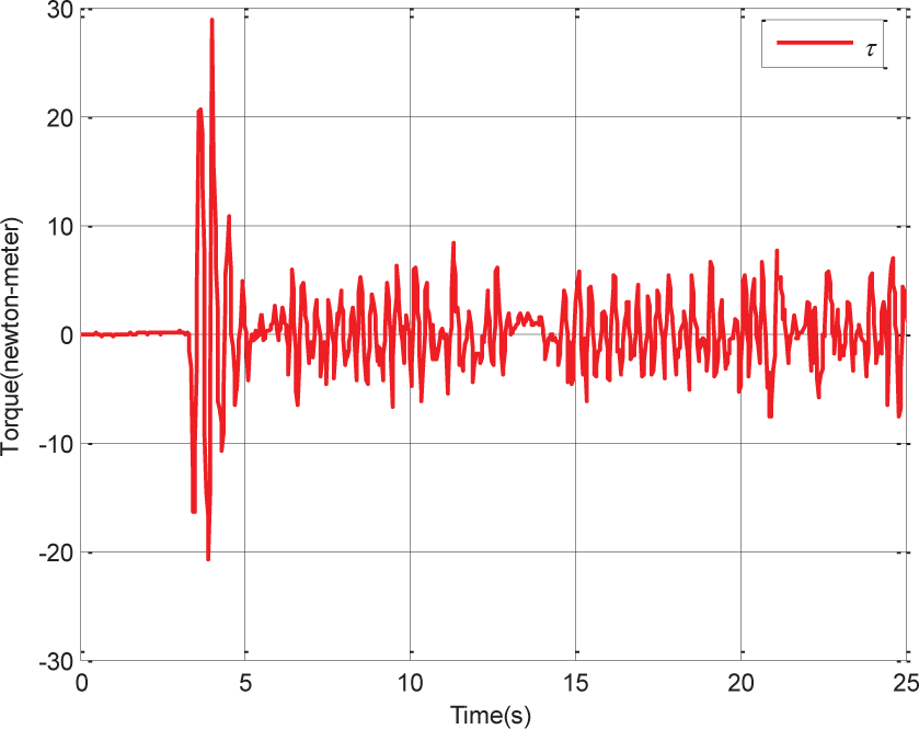
Control torque of the motor for the RTP robot on the wire with interference
Five seconds into the experiment, the RTP robot was pushed. Its roll angle increased to about 6°. Within about 3s, the robot returned to its initial position. The curve was similar to the ones in Figures 16 and 26. This showed the robot to be capable of recovering from interference.
Disturbing the RTP robot when it was moving and balancing it on the flexible wire returned it to a state of equilibrium after a moment of attitude adjustment. This showed that the RTP robot is robust.
Figure 27 shows a group of screenshots from the RTP robot experiment. The RTP robot moved on the wire safely from one end to the other - this is the ideal performance of our RTP robot.

Moving on the wire when subject to human interference
8. Conclusion
The present article discusses a wire-moving robot and the nonlinear controller that was established for use with it. This robot showed stable equilibrium control on a rigid rail and flexible wire. Its two-wheeled structure is an imitation of human feet and it was found to remain stability in the direction of travel. Its stability left-to-right was controlled by balancing poles. As in actual tightrope walking, the pole has two different movements, rotation and translation. However, it is difficult to imitate the flexible arm of a human using mechanical devices. Here, a parallelogram structure was used instead. In this device, the translation of the short pole was coupled with that of the rotational pole. Under these conditions, though the rotational pole does the bulk of the balance control, the movement of the centre of mass can be affected by either pole.
A computer simulation was performed on the rigid rail, and the same experiments were carried out using robot prototypes. Both robots showed the nonlinear controller designed using the partial feedback linearization control method to be effective. The results of these experiments were consistent with those of the simulations, as were those of the anti-interference experiment. In the experiments involving a flexible wire, if the wire shook heavily, the RP robot would fall off. This is also why so many people cannot walk tightropes. While the RTP robot succeeded in moving on the flexible wire. In conclusion, a wire-moving robot capable of moving on a flexible wire was designed, and an internal law of tightrope walking was proposed.
Footnotes
9. Acknowledgements
Our work is supported by the National Natural Science Foundation of China (grant no. 61105103) and the Beijing Natural Science Foundation (grant no. 4132032).