
Abstract
Recently, artificial neural networks have been used to solve the inverse kinematics problem of redundant robotic manipulators, where traditional solutions are inadequate. The training algorithm and network topology affect the performance of the neural network. There are several training algorithms used in the training of neural networks. In this study, the effect of various learning algorithms on the learning performance of the neural networks on the inverse kinematics model learning of a seven-joint redundant robotic manipulator is investigated. After the implementation of various training algorithms, the Levenberg-Marquardth (LM) algorithm is found to be significantly more efficient compared to other training algorithms. The effect of the various network types, activation functions and number of neurons in the hidden layer on the learning performance of the neural network is then investigated using the LM algorithm. Among different network topologies, the best results are obtained for the feedforward network model with logistic sigmoid-activation function (logsig) and 41 neurons in the hidden layer. The results are presented with graphics and tables.
Introduction
The inverse kinematics problem is one of the most important problems in robotics. Fundamentally, it consists in finding the set of joint variables to reach a desired configuration of the tool frame. Computer based-robots are usually acting in the joint space, whereas objects are usually expressed in the Cartesian coordinate system. In order to control the position of the end-effector of a robotic manipulator, an inverse kinematics solution should be established to make the necessary conversions. This problem usually involves a set of nonlinear coupled, algebraic equations. The inverse kinematics problem is especially complex and time-consuming for redundant types of robotic manipulators [1,2].
In the literature, inverse kinematics solutions for robotic manipulators are drawn from various traditional methods such as algebraic methods, geometric methods and numerical methods. Neural networks have also become popular [3–6].
Intelligent techniques have been one popular subject in recent years in robotics as one way to make control systems able to act more intelligently and with a high degree of autonomy. Artificial neural networks have been widely applied in robotics for the extreme flexibility that comes from their learning ability and function-approximation capability in nonlinear systems [2]. Many papers have been published about the neural-network-based inverse kinematics solution for robotic manipulators [7–14]. Tejomurtula and Kak presented a study based on the solution of the inverse kinematics problem for a three-joint robotic manipulator using a structural neural network which can be trained quickly to reduce training time and to increase accuracy [7]. Xia et al. presented a paper about formulating the inverse kinematics problem as a time-varying quadratic optimization problem. For this purpose they suggested a new recurrent neural network. According to their studies, their suggested network structure is capable of asymptotic tracking for the motion control of redundant robotic manipulators [8]. Zhang et al. used Radial Bases Function networks (RBF) for the inverse kinematics solution of a MOTOMAN six-joint robotic manipulator. They used the solution to avoid complicated traditional procedures and programming to derive equations and programming [9]. An adaptive learning strategy based on using neural networks to control the motion of a six-joint robot was presented by Hasan et al. Their study was implemented without explicitly specifying the kinematic configuration or the working-space configuration [10]. Rezzoug and Gorce studied the prediction of finger posture by using artificial neural networks based on an error backpropagation algorithm. They obtained lower prediction errors compared to the other studies in the literature [11]. Chiddarwar et al. published a paper based on the comparison of radial-base functions and multilayer neural networks for the solution of the inverse kinematics problem for a six-joint serial robot model, using a fusion approach [12]. Zhang et al. presented a paper about the kinematic analysis of a novel 3-DOF actuation-redundant parallel manipulator using neural networks. They applied different intelligent techniques such as multilayer-perception neural network, Radial Bases Function neural network and Support Vector Machine to investigate the forward kinematic problem of the robot. They found that SVM gave better forward kinematic results than other applied methods [13]. Köker et al. presented a study based on the inverse kinematics solution of a Hitachi M6100 robot based on committee-machine neural networks. They showed that using a committee-machine neural network instead of a unique neural network increased the performance of the solution; in other words, the error was decreased [14].
A neural network's working principle is based on learning from previously obtained data known as a learning or training set, and then checking the system's success using test data. The learning algorithm also affects the success of the neural network implementation significantly. In this paper, the effect of various learning algorithms, network types, activation functions and numbers of neurons in the hidden layer have been examined for the inverse kinematics solution of a seven-joint robotic manipulator. The results show that the Levenberg-Marquardt training algorithm, feedforward networks, logsig activation function and 41 hidden-layer sizes gave the best results for the inverse kinematics solution of the used robot model.
In the paper, section 2 provides a kinematics analysis of a Schunk LWA3 robot [15], section 3 outlines the neural-network-based inverse kinematics solution, section 4 describes training and testing, section 5 gives results and a discussion, and section 6 provides conclusions.
Kinematic analysis of Schunk LWA3 robot
A manipulator is composed of serial links that are connected to each other with revolute or prismatic joints from the base frame through the end-effector. The calculation of the position and orientation of the end-effector in terms of the joint variables is known as forward kinematics. In order to obtain forward kinematics of a robot mechanism in a systematic manner, one should use a convenient kinematics model. The Denavit-Hartenberg method, which uses four parameters, is the most common method to describe robot kinematics [16–18]. These four parameters can be described as ai−1, αi−1, d i , and θ i , which are the link length, link twist, link offset and joint angle, respectively. A coordinate frame is attached to each joint for the determination of DH parameters, and the zi axis of the coordinate frame points along the rotary or sliding direction of the joints [19,20].
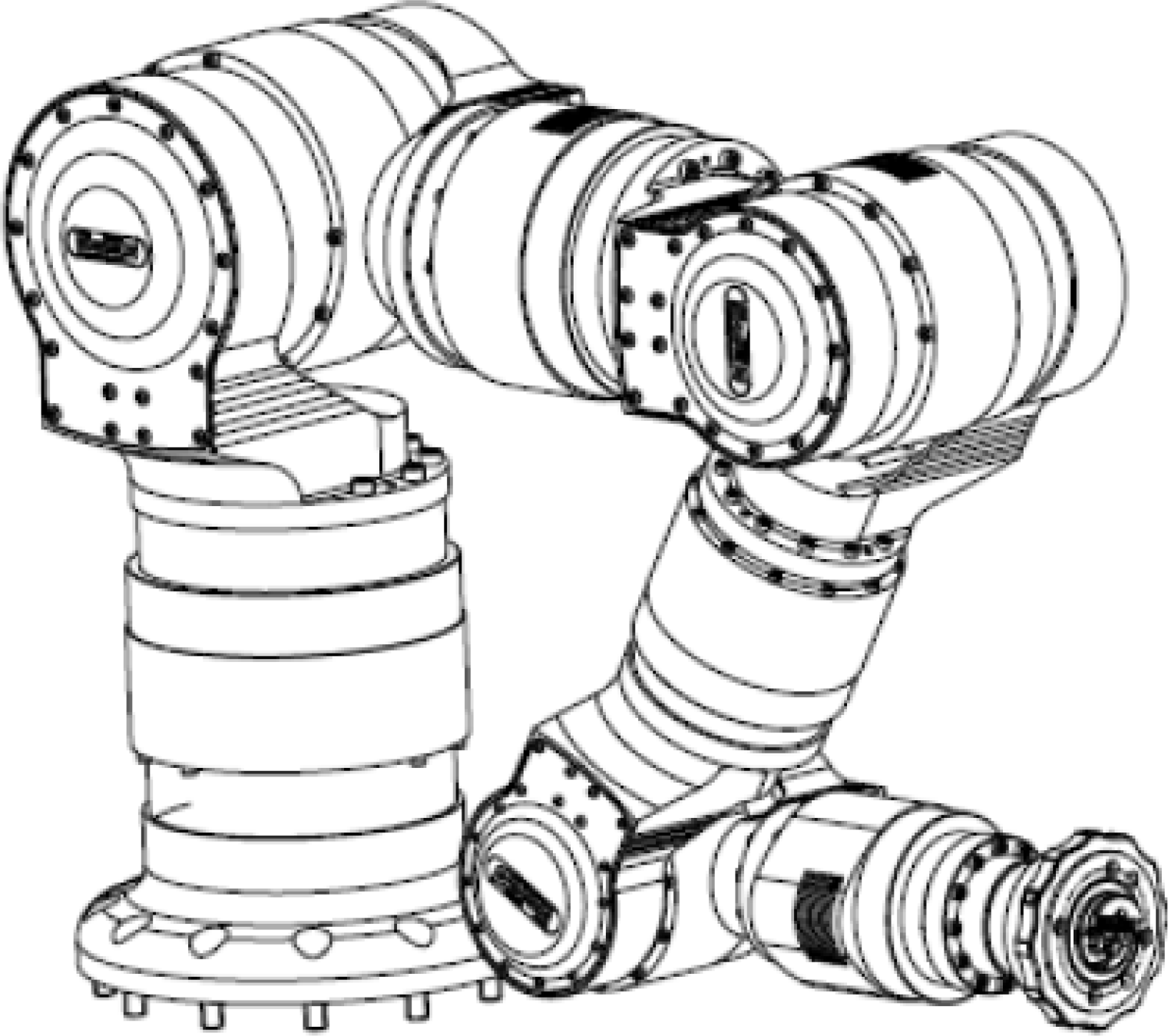
A seven-DOF Schunk LWA3 robot model has been used in this study, as shown in Figure 1. A 3-D view of the Schunk LWA3 robot is given in Figure 2. By using the above notations and Figure 1, the D-H parameters are obtained for this robot model as given in Table 1.

D-H parameters of the robot

The general transformation matrix i−1 i T for a single link can be obtained as follows:


In (1), (2) and (3), Rx and Rz present rotation, Dx and Qi denote translation, and ci, si, cαi−1, and sαi−1 are the short-hands for cosθ i , sinθ i , cosαi−1 and sinαi−1, respectively.
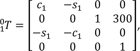
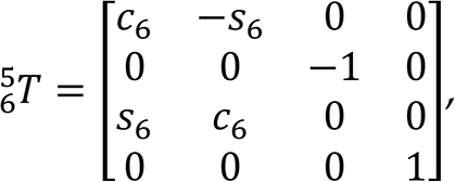
For the Schunk TWA3 robot, it is straightforward to compute each of the link transformation matrices using (1), as follows.


The forward kinematics of the end-effector with respect to the base frame are determined by multiplying all of the i−1 i T matrices as follows:

An alternative representation of e b T can be written thus:

In (12), n x , n y , n z , s x , s y , s z , a x , a y , a z refer to the rotational elements of the transformation matrix. p x , p y , and p z show the elements of the position vector.
For a seven-jointed manipulator, the position and orientation of the end-effector with respect to the base is given in (13).

All obtained notations after the calculations based on (13), are given in the Appendix.
By using (15)–(26) (see Appendix), the training, validation and test sets are prepared for the inverse kinematics model learning. All of these algorithms are implemented in MATLAB.
Neural networks are generally used in the modelling of nonlinear processes. An artificial neural network is a parallel-distributed information processing system. It stores the samples with distributed coding thus forming a trainable nonlinear system. Training of a neural network can be expressed as a mapping between any given input and output data set. Neural networks have some advantages, such as adoption, learning and generalization. Implementation of a neural-network model requires us to decide the structure of the model, the type of activation function and the learning algorithm [22, 23].
In Figure 3, the schematic representation of a neural-network-based inverse kinematics solution is given. The solution system is based on training a neural network to solve an inverse kinematics problem based on the prepared training data set using direct kinematics equations. In Figure 3, “e” refers to error – the neural network results will be an approximation, and there will be an acceptable error in the solution.
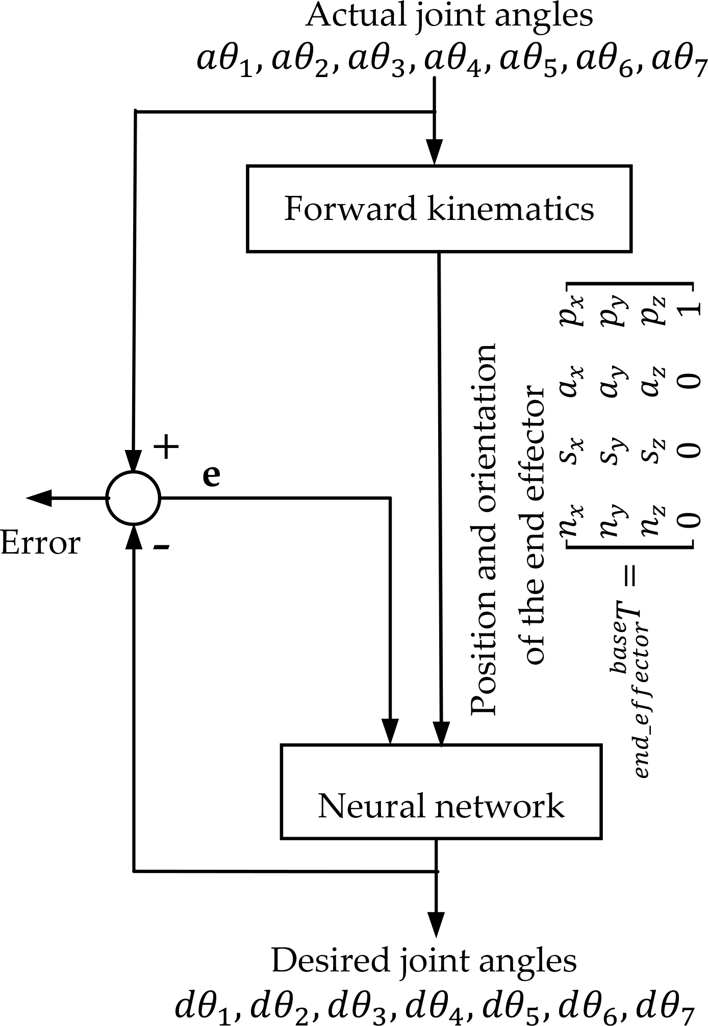
Neural-network-based inverse kinematics solution system [14]
The designed neural-network topology is given in Figure 4. A feed-forward multilayer neural-network structure was designed including 12 inputs and seven outputs. Only one hidden layer was used during the studies.

The neural network topology used in this study
The trained neural network can give the inverse kinematics solution quickly for any given Cartesian coordinate in a closed system such as a vision-based robot control system.
In this study, a fifth-order polynomial trajectory planning algorithm has been used to prepare data for training testing and validation sets of the neural network. The equation for fifth-order polynomial trajectory planning is given in (14):
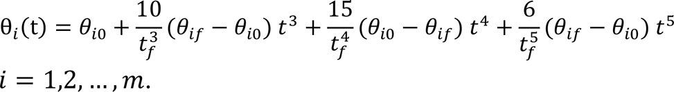
where θi(t) denotes the angular position at time t, θif is the final position of the ith joint, θi0 is the initial position of the ith joint, m is the number of joints, and tf is the arrival time from initial position to the target [24–28].
Some starting and final angular positions are defined to produce data in the work volume of the robotic manipulator. A sample trajectory is given in Figure 5 between 0 and 90 degrees for a joint.

A sample fifth-order polynomial trajectory
Twelve different training algorithms have been used in this study. The fundamentals of the 12 training algorithms are summarized in Table 2.
Different training algorithms used in this study

For the training 7000 data values corresponding to the (θ1,θ2,θ3,θ4,θ5,θ6,θ7) joint angles according to the different (n x , n y , n z , s x , s y , s z , a x , a y , a z , p x , p y , p z ) Cartesian coordinate parameters were generated by using the fifth-order polynomial trajectory planning given in (14) based on kinematic equations (15) to (26), given in the Appendix. A sample data set produced for the training of neural networks is given in Table 3. Here, the trajectory-planning algorithm has been used just to produce data between any given starting angular position and the final position, as mentioned above. Data preparation was done in a predefined area (robot working area). We tried to obtain well-structured learning sets to make the learning process successful and easy. These values were recorded in the files to form the training, validation and testing sets of the networks. Each 2380 of these data values were used in the training of neural networks, and 2310 were used in the validation of each neural network to see their success for the same data set. 2310 data values were used for the testing process as well. Training of the neural networks was completed when the error reached the possible minimum. The training and test results are given with details in the following section.
A sample data set produced for the training of neural networks

In this study, 12 training algorithms were used in the inverse kinematics model learning. The results of these algorithms are presented in Table 4. According to the table, the last five training methods – BFG, GDA, GDM, GD and GDX – are unsatisfactory. These are therefore neglected and not used in the graphical comparisons. The remaining seven training algorithms are compared.
Best performances for training, validation, and testing training times and number of epochs for different training algorithms

Best performances for training, validation, and testing training times and number of epochs for different training algorithms
Firstly, the comparisons are made by the number of epochs versus the mean squared error (MSE) values of the training, validation and testing. The graphical representations are given in Figures 6a, 6b and 6c, respectively. It is obvious from Figures 6a–c that the LM algorithm is the best one. The comparisons are then carried out by training time versus MSE values. These graphical comparisons are given for training, validation and test values in Figures 6d, 6e and 6f, respectively. The meanings of the lines used in these graphics are given in Figure 6g. Although 5433.6 seconds elapses for 1000 epochs during the training using LM, it is clearly seen in the three comparisons that the MSE value for the LM training algorithm is less than the MSE values of other algorithms around 65 seconds. According to these graphical representations, it is clear that the LM algorithm is a good and robust training algorithm for the inverse kinematics model learning of a robot. The MSE values of training, validation and testing according to the number of epochs for the LM algorithm is been given in the same graphic in Figure 7.

Comparison of training performances versus number of epochs for different training algorithms

Comparison of validation performances versus number of epochs for different training algorithms

Comparison of testing performances versus number of epochs for different training algorithms

Comparison of training performances versus time for different training algorithms

Comparison of validation performances versus time for different training algorithms
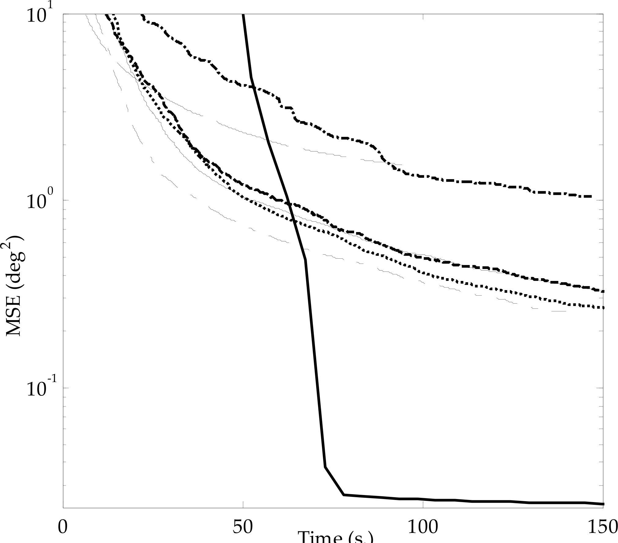
Comparison of testing performances versus time for different training algorithms
The meanings of the line styles in Figures 6a–f

Training, validation and testing values for LM algorithm
Since the LM algorithm is found to be significantly efficient, it is chosen for the analysis of the effect of various network types, activation functions and number of neurons in the hidden layer.
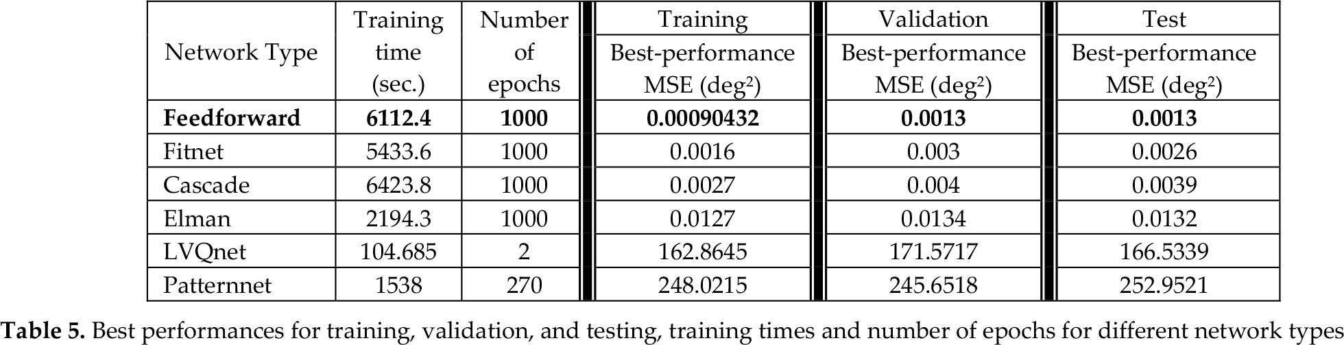
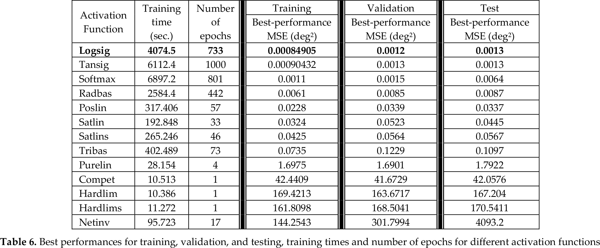
Six different network types, including 40 neurons in the hidden layer, were designed and examined by using the LM training algorithm and hyperbolic tangent sigmoid-activation function (tansig). The best results were obtained from the feedforward network model, as seen in Table 5. After this, 13 different activation functions were examined in the feedforward neural network model, including 40 neurons in the hidden layer, using the LM training algorithm. According to the results presented in Table 6, the logsig activation function was better than the others. Finally, the effect of different number of neurons in the hidden layer was analysed by using the feedforward neural network model with logsig activation function using the LM training algorithm. As is evident in Table 7, 41 neurons in the hidden layer gave the best result.
Best performances for training, validation, and testing, training times and number of epochs for different network types
Best performances for training, validation, and testing, training times and number of epochs for different activation functions
Best performances for training, validation, and testing, training times and number of epochs for different number of neurons in the hidden layer

Singularities and uncertainties in the robotic arm configurations are one of the essential problems in kinematics robot control resulting from applying a robot model. A solution based on using artificial neural networks was proposed by Hasan et al. [29]. The main idea is based on using neural networks to learn the characteristics of the robot system rather than having to specify an accurate robotic system model. This means the inputs of the neural network will also have linear velocity with the Cartesian position and orientation information to overcome singularities and uncertainties. Since the main focus of this paper is to investigate the performance of the various training algorithms in the neural-network-based inverse kinematics solution, however, this solution is not applied here.
This study has presented a performance evaluation of the various training algorithms and network topologies in a neural-network-based inverse kinematics solution for a seven-DOF robot. Twelve different training algorithms were analysed for their performances in the inverse kinematics solution for robotic manipulators. The LM training algorithm was found to be significantly the most efficient. It was evident that the LM algorithm was the fastest-converging algorithm and performed with high accuracy compared to the other examined training algorithms. Additionally, 13 different activation functions were examined during the study. The LM training algorithm was the fastest-converging one since it reached the lowest MSE value, around 65 seconds. In conclusion, the feedforward neural network model consisting of 41 neurons in the hidden layer with logsig activation function using the LM algorithm is successful for the inverse kinematics solution for a seven-DOF robot. As a future study, these training algorithms with a neural network could be examined on a real robotic manipulator, including hardware and software implementation of the solution scheme. Linear velocity could also be used as input of the neural network together with Cartesian position and orientation information, to overcome singularities and uncertainties.
Footnotes
Appendix