
Abstract
In this paper, we propose a computational trajectory generation algorithm for swarm mobile robots using local information in a dynamic environment. The algorithm plans a reference path based on constrained convex nonlinear optimization which avoids both static and dynamic obstacles. This algorithm is combined with one-step-ahead predictive control for a swarm of mobile robots to track the generated paths and reach the goals without collision. The numerical simulations and experimental results demonstrate the effectiveness of the proposed free-collision path planning algorithm.
Introduction
Motions planning of multiple mobile robots has been the subject of considerable research effort over recent years (see the references [10, 25, 31] and the references therein). In fact, a set of mobile robots can perform some tasks more efficiently and robustly than an individual robot. Moreover, the ability of mobile robots to navigate safely and avoid static and dynamic obstacles is necessary for many real world applications. Collision-free Paths Planning Methods (PPMs) require, in dynamic environments, dynamic collision avoidance algorithms. PPMs are more difficult to use in dynamic as opposed to static environments. We refer the reader to [12] for various complex algorithms proposed to solve this problem. In addition to their applications to mobile robot navigation, collision-free PPMs have been used successfully in fairly varied areas such as animation and graphics, intelligent transportation, and aerospace engineering. Collision-free PPMs are heavily based on a collision detection system dealing with the problem of checking whether or not two objects overlap in space.
Many methods have been proposed in the literature dealing with obstacle avoidance for robotics (see for instance the excellent book [17] and the references therein). The well known methods among them are the so-called Reactive Approaches, which have been used successfully for many years. They have been proposed for path generation for a single mobile robot (see for instance [12]). They are also known as local planning algorithms (LPA) [17]. During the last two decades, many authors extended some of them to multiple mobile robots (see for instance [3]). Among these approaches, we find the potential field approach [15, 16], the vector filed histogram [4, 10], the curvature method [27], and the dynamic window approach [11]. The main advantage of reactive methods is the fact that they are suitable for real-time navigation in unknown environments. These approaches use only sensor information (local navigation algorithm). However, the major drawbacks of these methods are: 1- the local minima where the robots are trapped; 2- the smoothness of the robot motion is not ensured.
In global planning algorithms, the information process of the environment is acquired partially before starting to use PPMs. Some of them have been developed and applied to mobile robot navigation in indoor or outdoor partially-known environments. A partially-known environment means that the position of walls or the topology of the scene (halls, walls and corridors) are known beforehand. We state and discuss in the following lines some existing papers [1, 14, 18, 24] that have studied situations with partially-known environments. In [1], the authors aimed to develop a control algorithm to command and manage a swarm of mobile robots for transshipment in harbors, airports and marshalling yards. They have designed an environment model of the scene where the algorithm has been implemented. The model contains a topological and geometrical representation of the environment where walls, routes and crossing are composed of cells. The known or unknown (static and dynamic) obstacles have also been taken into account online by the proposed scheme for avoidance capabilities. In [14], the authors have designed an autonomous mobile robot to clean floors for building maintenance where the environment is known a priori. The authors in [24] have realized a semi-autonomous navigation module for a robot wheelchair. The user of this wheelchair can execute the local manoeuvres algorithm in a narrow and cluttered space, as well as in a cluttered wide area. A climbing mobile robot has been designed in [18] for automatic wall inspections. The most important features to be inspected by the proposed mobile robot [18] are the rate of collision, detection of leaks, cracks and crumbling parts. These kinds of inspections are useful especially for the structure of buildings and in general for the safety of the environment. The topology of the space to be inspected is known in advance and the robot is able to navigate along different directions of the wall while avoiding different obstacles due to the structure of the building.
Furthermore, many authors have used collision-free PPMs to control multiple robots to maintain a given formation during the movement (see for instance [2, 7, 19]. In [19], the authors combined a collision-free PPM with a back-stepping controller and applied it to a dynamic model of a multiple robot navigation function to a team of holonomic and nonholonomic mobile robots. However, they assumed that the environment is known and stationary. The work in [2] proposed an obstacle avoidance algorithm based on fast speed generation in dynamic environments. If the generated speed does not belong to a required interval, then a set of acceleration (or deceleration) of robot's movement is provided. These adjustable accelerations represent the collision-free trajectories for the mobile robot. The algorithm has high computational complexity. In [7], graph theory is used to generate the collision-free path for each robot.
In our present work, an online path planning algorithm for multiple mobile robots is obtained using convex optimization with inequality constraints. The path of each robot is planned based on the position of static and dynamic obstacles in the neighborhood. Each robot considers the other robots as moving obstacles. Note that the proposed algorithm can be used for centralized control systems or decentralized control systems (distributed control systems). Knowing that centralized control systems solve a single optimization algorithm with constraints for the entire team, this will require significant computation according to the size of the team. For the distributed control of multiple mobile robots, each robot's behaviour is affected by its neighbour's actions. The proposed algorithm performs an online path planning with global convergence and is applied to nonholonomic wheeled mobile robots. Our main aim in this work is to remove the major drawbacks of the LPA (local planning algorithms), namely, the local minima problem and the smoothness of robot motion. Using a convex constrained minimization problem, we do not encounter the local minima problem, and the special structure of our non-overlapping scheme allows us to prove mathematically the smoothness of the robot motion.
The paper is organized as follows. Section 2 is devoted to the mathematical framework, namely, the description of the non-overlapping scheme. In Section 3, we prove the smoothness of the robot motion. Section 4 contains an application to swarm mobile robots of the abstract scheme described in Section 3. The numerical simulations and experimental results are gathered in Section 5. A brief conclusion ends the paper.
Collision-free path planning
In this section we present an algorithm allowing us to handle contacts between wheeled mobile robots and obstacles. For more applications of this algorithm to real life problems we refer to [20, 21].
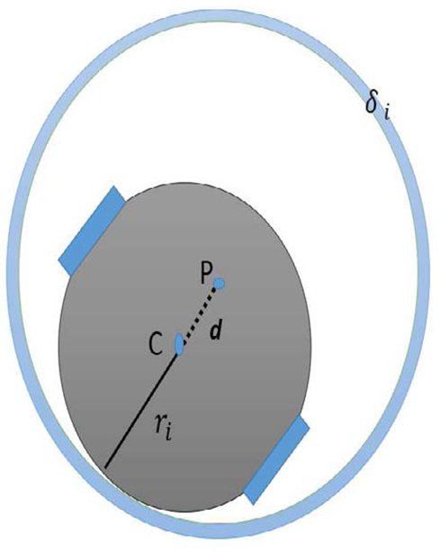
Consider N1 mobile robots (or agents) and N2 obstacles (static and/or mobile) with arbitrary forms. Robots and obstacles are immersed in rigid disks with different radii R i , i = 1, ···, N1 + N2. The safety distance is denoted by δ i > 0 as Figure 1 shows.
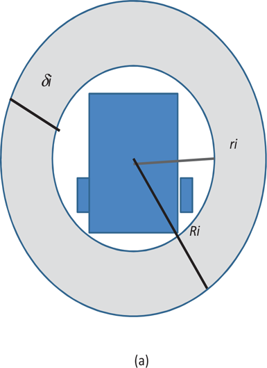
Mobile robot representation inside the safety disk

Obstacle representation inside the safety disk
In the case of circular mobile robots (or obstacles), the safety distance is: δ i = Ri − ri, where ri is the radius of the mobile robot (or obstacle). Note that a robot or an obstacle i having a general shape (see Figure 1–b) is first immersed in a disk with radius ri and this disk is then immersed in a safety disk with radius Ri. So, the safety distance in this case is also given by δ i = Ri − ri.
The purpose is to simulate the motion of the mobile robots inside a given domain Ω in ℝ2 during an interval time [0, T] and subject to the static and/or dynamic obstacles.
To do that, we consider the configuration vector q = (q1, q2, ···, qN) ∊ ℝ2N (N ∊ ℕ) where qi is the centre of the safety disk i with coordinates (

where Dij(q) = ‖qi − qj‖ − (Ri + Rj) is the distance between the safety disks i and j. From a mathematical point of view, collision avoidance between safety disks i and j at time t means the non-negativity of the distance Dij(t). Thus, starting from an admissible configuration q(t) at time t, we want to ensure the admissibility of the configuration vector q(t + h) after a small value of unit of time h > 0. For this aim, we define the set of admissible velocities ensuring the non-overlapping of safety disks during all the time interval [0, T]:

where ∇Dij(q) is the gradient of the distance function Dij(q). Indeed, if we are given an admissible configuration

By taking the real velocity

and so by (2.3) we obtain Dij(q(tn + h)) ≥ 0, that is, q(tn + h) ∊ Q.
Let U(q) be the desired velocity of all mobile robots and obstacles. For the static obstacle the desired velocity is always assumed to be zero. To avoid the overlapping of all the safety disks which ensures the free-collision of robots and obstacles, we propose the following scheme:
Given an admissible configuration

where Wn+1 is the solution of the convex constrained optimization:
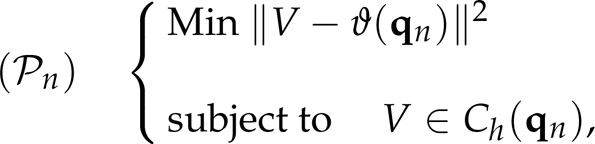
that is, ‖Wn+1 − ϑ(
The main characterizations of the algorithm defined in the previous section, which distinguish it from other methods, are: 1- the smoothness of the motion of each robot, that is, the trajectory generated by the algorithm is continuous, and 2- no collision between the safety disks of robots and obstacles. Indeed, if we are given a time horizon T, we fix N ∊ ℕ and we divide the interval time I := [0, T] into N subintervals with equal length

Here Proj S (x) stands for the metric projection of the point x ∉ S on the closed set S, that is, u = Proj S (x) provided that u ∊ S and ‖u − x‖ = infs∊S ‖s − x‖.
The algorithm (Pn) is well defined due to the closedness and convexity of the set Ch(

Clearly, qN is defined over I,

Observing that K(

which can be rewritten as

In order to prove the convergence of the sequence of functions (qN) N , we rewrite the previous equality in terms of the normal cone in the sense of convex analysis, that is,

with qN(0) =

The above inclusion 3.2 is called the Sweeping Process with Perturbation introduced and studied by Moreau [22] and extended in different ways by many authors (see for instance [5, 6, 9] and the references therein). Using the techniques developed in [6, 9], the author in [30] proved in Theorem 4.5, the uniform convergence of the sequence qN satisfying (3.2) to a unique absolutely continuous function q such that
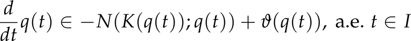
with q(0) ∊ Q0, q(t) ∊ K(q(t)), ∀t ∊ I. The author in [30] also proved in Proposition 4.7 that q(t) ∊ Q0, ∀t ∊ I. This proves that the limit trajectory q satisfies our requests, that is, q is continuous and is admissible in Q0 during the time interval I, which means that the motion of the robots will be smooth and with collision-free trajectories.
In this section we present a real life application of the numerical scheme (2.4) described previously to path tracking of the mobile robots.
Description of Wheeled Mobile Control (WMR)
The mobile robot used in this work is a simple unicycle mobile robot type shown in Figure 3.
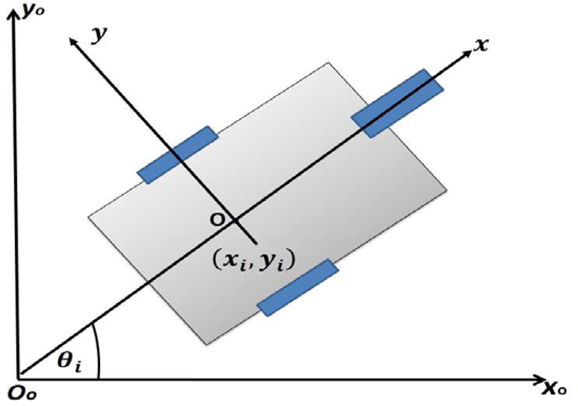
Wheeled mobile robot
The kinematic model for i th WMR is (see for instance[23, 26]):

where
A configuration of the robot i is given by:
The commands of the ith differential drive mobile robot are the velocities of the right and the left wheels

and

where L is the distance between two wheels. The kinematic model (4.1) of the WMR becomes:

The kinematic model presents the nonholonomic constraint which is given by:

This constraint means that the robot path is tangent to the main axis of the robot.
It is known that in order to design a trajectory tracking controller via feedback a coordinates transformation is used to overcome the noncontrollability of the nonlinear model (4.1). This transformation is given by (see for instance [26]):
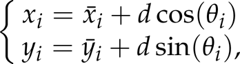
with d ≠ 0. These coordinates represent the Cartesian coordinates of a point located along the axis of the WMR at a distance d from the center of the line connecting the contact-point of the wheels with the ground. Hence, the center
The effective center and the effective radius of the safety disk
The derivatives of the new model of the WMR are:

The nonlinear model of the mobile robot can be written under matrix form as:
where

and

In this work, we consider the problem of tracking a reference trajectory given by the equation:

for the ith mobile robot. The reference trajectory
The tracking control problem is to find for the ith robot a suitable control vector Ui(Zi; t) to drive the mobile robot (4.4) to track precisely the desired trajectory (4.5).
The goal of the tracking control problem of the ith mobile robot is to minimize the cost function given by:

where ei(t) = Zi(t) − Zi,ref (t) is the tracking error, Q is a positive definite matrix, R is a positive semi-definite matrix and h is the prediction horizon. The desired trajectory is specified by a smooth vector function Zi,ref(t) for t ∊ [0, T]. Note that T is the final time needed for all the robots to reach all the targets. The problem comprises elaborating a control law Ui(Zi, t) that improves tracking accuracy at the step t + h, where h > 0 is a prediction horizon, such that Zi(t + h) tracks Zi,ref (t + h). That is, the tracking error is defined by:

A simple and effective way to predict the influence of Ui(t) on ei(t + h) is to write its first order Taylor expansion as follows:

In order to find the current control Ui(t) that improves tracking error at the next step and to avoid the computational burden, the expression of the above-predicted tracking error is used in the objective function (4.6). Therefore, the unique control signal U
i
* that minimizes Ji, obtained by setting

Tracking performance: For simplicity, let R = 0, equation (4.8) becomes:

and we can show easily that the mobile robot model with the feedback control (4.9) leads to:

The error dynamics (4.10) is linear and time-invariant. Thus, the proposed controller that minimizes the one step ahead predicted tracking error naturally leads to a special case of input/state linearization. The advantage of this controller with regard to the linearization method is a clear physical meaning of maximum and minimum when saturation occurs. Note that the tracking error dynamic (4.10) is stable for any h > 0.
Simulation Results
This section presents the results of the numerical simulations using MATLAB to show the application of the collision-free path planning algorithm described in Section 2 with a one-step-ahead predictive controller. To verify the effectiveness of the proposed algorithm, we have set up a simulation with two robots and different static obstacles. The robots are represented as small filled disks (Rob. 1 as black and Rob. 2 as blue).
The objective is to drive each mobile robot (Rob. 1 and Rob. 2) towards its corresponding targets (Targ.1 and Targ.2) without collision with the obstacles and the other robot. Each robot uses the reference trajectory induced from the collision-free path planning algorithm (2.4) and generates the control vector U i to be applied to the robot i using the one-step-ahead predictive control.
We have two different situations in our numerical simulations. The first one is the case of obstacles included in safety disks and without walls. The second one is the case of obstacles as walls.
Case 1: Without walls
The initial configuration

where
q10 =
q20 =
qobs10 =
qobs20 =
qobs10 =
The position of the targets are:
q
targ1
=
q
targ2
=
The radii used in the simulations are: r1 = r2 = 0.2; robs1 = robs2 = 0.7; robs3 = 1.2; δ1 = δ2 = 0.05; d = 0.05.
The first graph in Figure 5 shows the tracking performance of the proposed algorithm in mid-path. Two robots, which are represented by two small disks, are going towards their target and avoid the first obstacle in their path.

Mid-path planning and obstacle avoidance of two mobile robots
The second graph in Figure 5 shows the tracking performance of the proposed algorithm. Two robots reach the targets without colliding neither with the last obstacle nor with each other. Indeed, at the end of the path, Rob. 1 encounters two obstacles: static obstacle which is the third obstacle and the dynamic obstacle which is Rob. 2. Additionally, the robot Rob. 2 meets two obstacles: a static obstacle which is the third obstacle and a dynamic obstacle which is Rob. 1. The figure shows clearly how robots Rob. 1 and Rob. 2 avoid each other and how they avoid the third obstacle during their way to the targets respectively.
The three graphs in Figure 6 show the case of two mobile robots with two static obstacles. These two mobile robots meet at the mid-path and the graphs show clearly how they avoid collision. Note that Rob. 1 has slowed down its speed letting Rob. 2 follow its path towards Targ. 2.

Navigation performance of two-WBR: 1- meeting of two mobile robots at the mid-path. 2- Obstacle avoidance performance. 3- Arriving at the targets.
Case 2: Walls as obstacles
The environment in this simulation contains two parallel walls as Figure 7 shows. The initial configuration

Tracking performance of two mobile robots with wall obstacles
q10 =
q20 =
The position of the targets are:

The radii used in the simulations are: r1 = r2 = 2.5.
Each robot reaches its corresponding target without collision neither with the walls and nor with the other robot (see Figure 7). We also have to point out the smoothness of the motion of both robots due to our proposed algorithm.
In this subsection, we focus on the implementation of our algorithm to the motion of three mobile robots. The experiments have been conducted using TOSHIBA laptops (Qosmio) with Intel Core i7 processors. MATLAB software has been used with a Bluetooth communication system. The platform used in this work is Khepera III 8)(made by K-TEAM [32]), which is a differential drive mobile robot with a circular shape 12 cm in diameter. It senses its environment using five ultrasonic sensors and 11 IR sensors (see Figure 9). In our lab experiments, we used only the eight IR sensors corresponding to labels 0 to 7 in Figure 9. Each IR sensor has a range of measurements from 5 mm to 200 mm. To compute the distance between the robot i and the existing obstacles, we first read all the sensors for robot i, IR i s s = 0, …, 7, and we take the maximum over all the sensors,

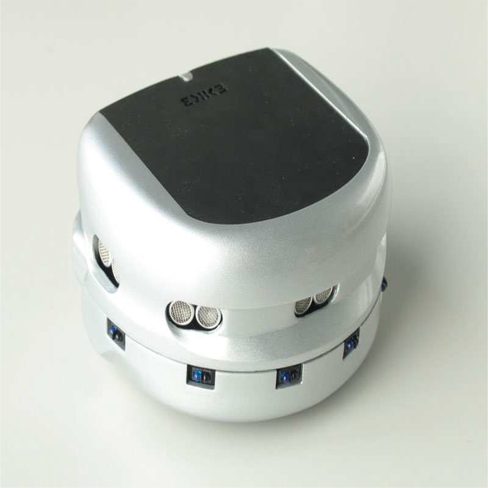
Khepera-III
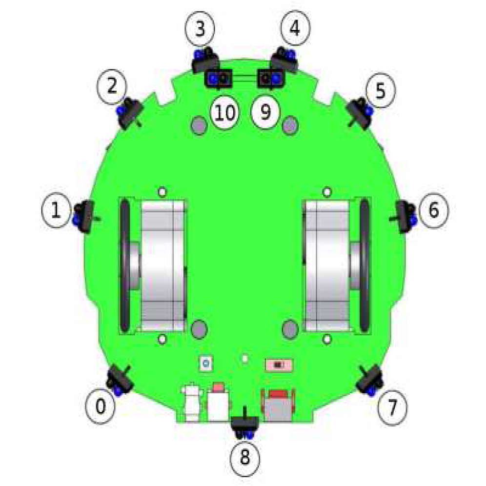
Bottom view of the IR sensors in Khepera-III
If IRi is greater than a given threshold, we deduce the presence of at least one obstacle. For a detected obstacle j we associate a reading number IRi,j which is the reading number of the sensor detecting that obstacle. Once the values IRi,j are collected, we convert them to distances via the function
The implementation of the algorithm is conducted on three different laptops which are connected to three Khepera robots via Bluetooth. The proposed navigation algorithm needs, for its implementation, the (x, y)-position relative to the world frame of all obstacles (both mobile and static). We denote by
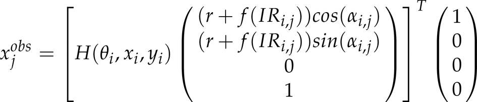
and

Here H (θ i , x i ,y i ) is the homogeneous transformation matrix given by

where θ
i
is the orientation of Robot i,

Detection of Obstacle j by Robot i
The implemented algorithm used in our lab experiments is described as follows:

Real-time obstacle avoidance for Robot i
We summarize the constants used in all our lab experiments in the following table:
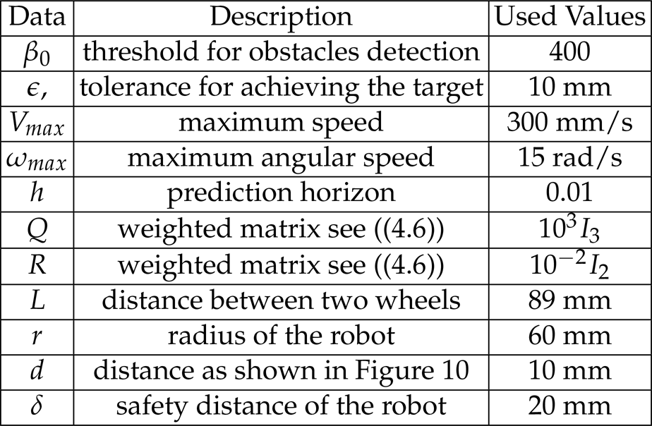
In our lab experiments we produced three scenarios as follows:
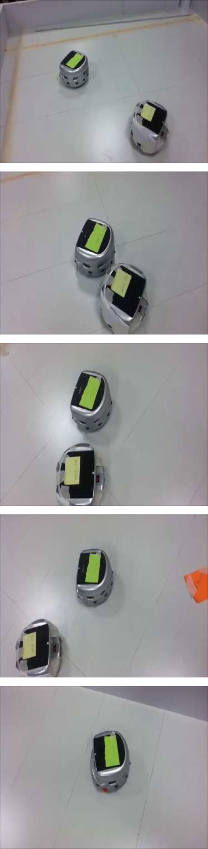
Scenario 1: One mobile robot and a static obstacle. In this scenario we examined the case when the mobile robot started from a given point going to a final target and avoiding a fixed obstacle which is situated in the mid-path as shown in Figure 11. The video showing this scenario is uploaded on YouTube at http://youtu.be/vrlxi7XHlrI. Scenario 2: Two mobile robots. In this scenario we examined the case when two mobile robots started from two different starting points, going to their final targets, and avoiding each other as shown in Figure 12. The video showing this scenario is uploaded on YouTube at http://youtu.be/38wTGuWkkKI. Scenario 3: This scenario is more complicated than the previous ones. We put three mobile robots at three different starting points, going to their final targets, and avoiding each other as shown in Figure 13. We point out that the starting points were very close to each other in order to get the more complicated scenario. The video showing this scenario is uploaded on YouTube at http://youtu.be/ZAwln4FlQf0.
Snapshots for Scenario 1
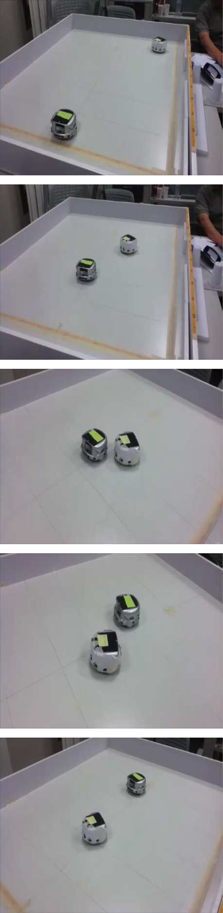
Snapshots for Scenario 2

Snapshots for Scenario 3
The computation time of the algorithm in the real world experiments depends on the presence and on the number of obstacles. Indeed, in the case of no obstacles, the time processing has been evaluated to be 0.3233 seconds. However, in the presence of one mobile obstacle (Scenario 1) the algorithm reads the values of sensors (IRs, s = 0 to 7), determines the nearest obstacles, and calls an external function to estimate the position of these surrounding obstacles. Therefore, the time processing of the algorithm increases to 1.8 seconds instead of 0.3233 seconds. We point out that the processing time for our algorithm in all the implementations is relatively high which is due to the use of MATLAB under Windows 8, which is known for its slowness in the implementation relative to other softwares such as C++.
This paper presents a collision-free path planning using nonlinear optimization combined with one-step-ahead predictive controller. The proposed collision-free path planning algorithm is an online path planning with a global minimum. The simulations and experimental results showed the effectiveness of this algorithm, namely, overcoming the local minima problem and smoothness of robot motion. Indeed, it was desired (in both simulations and lab experiment) to control the mobile robots smoothly to their desired targets without collisions between them and avoiding the static obstacles.
The proposed algorithm can be used efficiently in many applications where the environment is partially known. For instance, in building for maintenance and inspection, hospitals and warehouses for material handling. In this case, the direction or velocity of each mobile robot can be determined precisely in a given region. The algorithm can provide the optimal velocity to move the mobile robot from the current position to the next free position without colliding with walls or with any other obstacles (static or dynamic). For a completely unknown environment, the sensors are used to estimate the position of the obstacles which will be inserted in our algorithm to determine the next free position in the scene. Therefore, the optimal velocity can be calculated using the proposed scheme to navigate the mobile robot to the next position from the current one.
In the simulations, good tracking performances and navigation without collision have been obtained in the presence of the obstacles. However, in this case the positions of obstacles are known exactly and we therefore have no need for a localization algorithm. For the experimental part, to perform the proposed algorithm, localization and position estimation of obstacles algorithms have been included. The tracking performances and navigation of the wheeled mobile robot, in an unknown environment with static and dynamic obstacles, are good and robust against the uncertainties induced by the infrared sensors.
Footnotes
7.
The authors extend their appreciations to the Deanship of Scientific Research at King Saud University for funding the work through the research group project No. RGP-VPP-024.