Path-tracking Algorithm for Aircraft Fuel Tank Inspection Robots

Abstract

A 3D path-tracking algorithm based on end-point approximation is proposed to implement the path traversal of robots designed to inspect aircraft fuel tanks. Kinematic models of single-joint segments and multiple-joint segments were created. First, each joint segment of the path was divided into many equal sections and the rotation angle was computed. The rotation angle was found for the plane determined by one divided point and the secondary terminal joint segment. Second, the shortest distance search strategy was used to calculate the bending angle of the joint segment. The main advantage of the algorithm was that only the terminal joint segment variables needed to be solved, the joint variables of other joint segments were copied from the adjacent front-end joint segment variables in turn. Finally, evaluation indexes of path tracking performance were proposed to evaluate the effect of the algorithm. Simulations of planar and space path tracking were carried out using MATLAB, and the effectiveness and stability of the tracking algorithm were verified.

1. Introduction

In the field of civil aviation aircraft maintenance, fuel tanks are usually checked manually for leaks or corrosions, and air personnel must enter the aircraft fuel tanks. However, the operating space is narrow, and the fuel tank is a flammable and explosive environment where the fuel mixes with fuel-gas. As such, fuel tank maintenance is highly labour-intensive, inefficient and risky. The crews must follow the Aircraft Maintenance Manual (AMM) strictly. Robotic technology may improve performance. This paper presents a design for an aircraft fuel tank inspection robot (AFTIR) with a continuous structure to assist crews in carrying out inefficient and risky fuel tank inspection operations.

Unlike robots that are constructed in a series of rigid links, continuum robots move by bending and rotating, in structures meant to resemble tentacles or snakes [1]. The fundamental differences between discrete, serpentine and continuum robot devices have been defined [1]. Continuum robots have attracted the interest of many researchers because of their dexterous and innately compliant bodies [2]. Continuum robots can flexibly change their shape by bending into smooth, continuous curves. In this way, they may function well in narrow workspaces with strong spatial constraints.

Several research teams have studied topics related to continuum robots, most of them in the medical field, especially minimally invasive surgery (MIS). Continuum robots designed to enter a given operative position have been proposed in previous studies [3–7]. These robots were driven by cables. Kinematics models have been built and analysed. One approach to compliant motion control that does not require the explicit estimation of interaction forces has also been presented in previous studies [8–11]. A continuum robot with a coupled tendon drive has been developed for use in the examination of human heart disease [12]. The authors presented a method of controlling a tendon-driven continuum manipulator by specifying the shape configuration. The basis for the control was a linear beam configuration model that transformed the beam configuration into tendon displacement by modelling the internal loads of the compliant system [13–14]. In three previous studies, a colon endoscope robot was developed for the examination of human colons [15–17]. Based on the analysis of continuum robots, a novel and simplified kinematics for cable-driven continuum robots was presented using a geometric analysis. The mapping relationships between simple joint drive space, joint space, and operation space were analysed, and the 3D workspace was introduced.

A hyper-articulated robot arm designed for assembly operations inside an aircraft wing-box has also been designed. It uses an actuator module composed of a shape memory alloy (SMA), whose structure can change [18–19]. The British OC company developed a continuum robot for the inspection of nuclear power plants. Its body consists of many structural units, and it is operated by a remote cable [20].

However, path tracking problems have not been addressed in the papers presented above. Robots that work in large aircraft fuel tanks with distributed ribs require a feasible tracking algorithm for given paths. The tracking problem for mobile robots can be simplified by treating the robot as a particle. However, when it comes to the continuum robot, we should ensure that the whole body moves along the path as closely as possible. Unfortunately, few studies have addressed path tracking issues for continuum robots.

A 3D path tracking approach based on endpoint approximation is proposed. The joint segment variables are calculated using this method. Evaluation indexes for path tracking performance are proposed for the evaluation of the effects of this algorithm. Simulation experiments show that it can track any given path effectively.

The structure of this paper is as follows. Section 2 provides an overview of the system structure of AFTIR and the prototype. Section 3 presents a kinematic analysis of the continuum robot. The path tracking algorithm is then presented in section 4 along with a concrete implementation. Section 5 describes the proposed evaluation indexes for the path tracking performance and the analysis of the path tracking simulation. It also provides a verification of the algorithm using experiments. The conclusions are summarized in section 6.

2. Structure analysis for AFTIR

AFTIR consists of a snake-like arm mechanism (SLA for short), a telescopic mechanism, a control system, and a mobile platform, as shown in Figure 1(a). The SLA mechanism consists of an SLA shell, an SLA, an actuation system, and an image perception module. The prototype is shown in Figure 2. The SLA consists of a number of serially connected identical 2-DOF cable-driven joint segments (JS for short). The actuation system consists of a distaff mechanism, DC motors, and a subsidiary body. The telescopic mechanism is composed of a linear module and a DC motor. The base of the SLA is fixed to the slider of the linear module. In this way, the SLA can perform translation motions along the linear module. The control system performs tasks such as path planning path tracking image processing, and information transmission.

Figure 1.

Structure of the AFTIR

Figure 2.

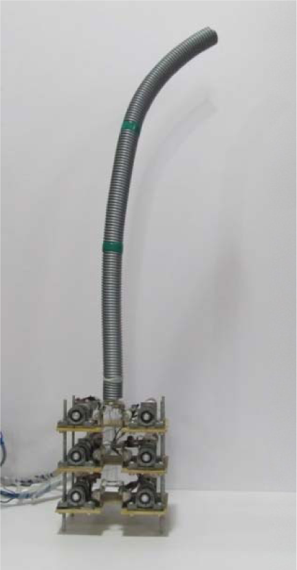
Prototype of the SLA mechanism

Each JS consists of a flexible backbone, a base disk, an end disk, several support disks, and four driving cables, as shown in Figure 1(b). As the base disk, the end disk and several support disks are connected by the flexible backbone at their centres, the motion characteristics are governed by elastic deflections of the backbone. For 2-DOF JS, the flexible backbone is made of glass fibres and its structure is designed so that it possess a very high tensional stiffness to prevent a twisting motion occurring around the backbone axis. As a result, the JS with the flexible backbone will only produce 2-DOF motions. To simplify the SLA analysis, all JS are assumed to be the same. The attachment points of the four driving cables are symmetrically arranged at 90° on both disks. The two driving cables are arranged at 180° and controlled by one motor. When the motor runs, the lengths of the two cables change inversely.

3. Kinematics of the AFTIR

3.1 Definition of the coordinate systems

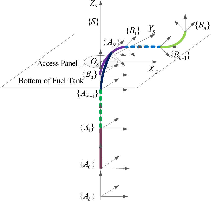
Four frames were introduced to establish the kinematic models. The system frame {S} is attached to the aircraft fuel tank access panel with its origin located at the centre of the access panel. The Zs axis is normal to the access panel and Xs axis is coincident with the minor axis of the access panel. Frame {A_b} is attached to the base of the telescopic mechanism.

Frame {A_j-1} is attached to the base disk of the j-th JS with its origin located at the centre of the disk, as in Figure 1(b) and Figure 3. The X_Aj-1 axis points to the first cable attachment point on the disk. The Y_Aj-1 axis points to the second cable's attachment point on the disk. Because the end disk of the j-th JS is closely connected to the base disk of the (j+1)-th JS, frame {A_j} can be considered as being attached to the end disk of the j-th JS. Similarly, the path of the JS frame {B_g} (g=0, 1, 2, …, n) is defined as shown in Figure 4. Let N be the number of the SLA JS and n be the number of the planned path JS. At the beginning of the program, the end of the SLA reaches Os, the origin of frame {S}, as shown in Figure 4.

Figure 3.

Kinematics of single JS

Figure 4.

Schematic diagram of coordinate systems

3.2 Forward kinematics of single JS

The 2-DOF bending motions generated by the j-th cable-driven JS with the flexible backbone can be described by two parameters: the rotation angle φR_j and the bending angle θ_Rj, as shown in Figure 3.

When the 2-DOF JS bends, the bending shape of the backbone is assumed to be circular with a constant arc length L. The bending plane formed by the flexible backbone arc O_AjO_Aj-1 is always perpendicular to the base disk plane. The angle between the bending plane and plane X_Aj-1O_Ai-1Z_Aj-1 is defined as the rotation angle φ_Rj, and the backbone deflection within the bending plane is described by the bending angle θ_Rj.

The purpose of the forward kinematics analysis is to find the pose that the JS end may assume based on the lengths of the four driving cables. Joint variables [φ_Rj, θ_Rj] are here used as the intermediate variables to simplify the analysis. It is easy to find the mapping between the lengths of the cables and the joint variables, as shown in equation (1).

$\{\begin{array}{l}\mathrm{\Delta }{l}_1=r{\theta }_{Rj}\cos {\phi }_{Rj}\\ \mathrm{\Delta }{l}_2=-r{\theta }_{Rj}\cos ({\phi }_{Rj}+\frac{\pi }{2})\\ \mathrm{\Delta }{l}_3=-r{\theta }_{Rj}\cos {\phi }_{Rj}\\ \mathrm{\Delta }{l}_4=r{\theta }_{Rj}\cos ({\phi }_{Rj}+\frac{\pi }{2})\end{array}$

(1) Here, Δl_i (i=1,2,3,4) represents the quantity of the change of the length about the i-th driving cable, and r is the radius of the graduated circle as determined by the four cable attachment points.

Assuming P_j is the position vector of the point O_Aj relative to frame {A_j-1}, then the following is true:

$P_j=\left(\begin{array}{c}{x}_{O_{Aj}}\\ y_{O_{Aj}}\\ z_{O_{Aj}}\end{array}\right)=\left(\begin{array}{c}\frac{L}{{\theta }_{R_j}}\cos {\phi }_{R_j}(1-\cos {\theta }_{R_j})\\ \frac{L}{{\theta }_{R_j}}\sin {\phi }_{R_j}(1-\cos {\theta }_{R_j})\\ \frac{L}{{\theta }_{R_j}}\sin {\theta }_{R_j}\end{array}\right)$

(2) The homogeneous transfer matrix ${\hspace{0.17em}}_{\hspace{0.17em}\hspace{0.17em}\hspace{0.17em}\hspace{0.17em}{A}_j}^{A_{j-1}}T$ of frame {A_j} with respect to {A_j-1} can be described using formula (3).

$\begin{array}{l}{\hspace{0.17em}}_{\hspace{0.17em}\hspace{0.17em}\hspace{0.17em}\hspace{0.17em}{A}_j}^{A_{j-1}}T=D(P_j)\cdot R_Z({\varphi }_{R_j})\cdot R_Y({\theta }_{R_j})\cdot R_Z(-{\varphi }_{R_j})\\ =\left(\begin{array}{cccc}c{\theta }_{R_j}{c}^2{\phi }_{R_j}+s^2{\phi }_{R_j}& c{\theta }_{R_j}s{\phi }_{R_j}c{\phi }_{R_j}-c{\phi }_{R_j}s{\phi }_{R_j}& s{\theta }_{R_j}c{\phi }_{R_j}& \frac{L}{{\theta }_{R_j}}c{\phi }_{R_j}(1-c{\theta }_{R_j})\\ c{\theta }_{R_j}c{\phi }_{R_j}s{\phi }_{R_j}-c{\phi }_{R_j}s{\phi }_{R_j}& c^2{\phi }_{R_j}+s^2{\phi }_{R_j}c{\theta }_{R_j}& s{\theta }_{R_j}s{\phi }_{R_j}& \frac{L}{{\theta }_{R_j}}s{\phi }_{R_j}(1-c{\theta }_{R_j})\\ -s{\theta }_{R_j}c{\phi }_{R_j}& -s{\theta }_{R_j}s{\phi }_{R_j}& c{\theta }_{R_j}& \frac{L}{{\theta }_{R_j}}s{\theta }_{R_j}\\ 0& 0& 0& 1\end{array}\right)\\ \end{array}$

(3) Where, sθ _{R j} is shorthand for sin θ _{R j} , cθ _{R j} is shorthand for cos θ _{R j} , s²φ _{R j} is shorthand for (sin φ _{R j} )², c² φ _{R j} is shorthand for (cos φ _{R j} )², and so on.

3.3 Kinematic analysis of multi-JS

After a number of identical 2-DOF joint segments are connected in series, the forward kinematics of the SLA can be derived. The homogeneous transformation from frame {A_f} to {A₀} can be written as follows:

${\hspace{0.17em}}_{A_f}^{A_0}T={\hspace{0.17em}}_{A_1}^{A_0}T\cdot {\hspace{0.17em}}_{A_2}^{A_1}T\cdot {\hspace{0.17em}}_{A_3}^{A_2}T\cdots {\hspace{0.17em}}_{\hspace{0.17em}\hspace{0.17em}\hspace{0.17em}\hspace{0.17em}{A}_f}^{A_{f-1}}T$

(4) ${\hspace{0.17em}}_{A_0}^{A_b}T$ is used to express the translation motion of the telescopic mechanism, and ${\hspace{0.17em}}_{A_b}^{S}T$ is known. The transfer matrix from frame {A_f} to {S} can be obtained as in formula (5).

${\hspace{0.17em}}_{A_f}^{S}T={\hspace{0.17em}}_{A_b}^{S}T\cdot {\hspace{0.17em}}_{A_0}^{A_b}T\cdot {\hspace{0.17em}}_{A_f}^{A_0}T$

(5)

4. Path tracking algorithm of the AFTIR

4.1 General concepts of aircraft fuel tank inspection

An AFTIR inspection of a fuel tank would take place as follows.

• (1)

The path is planned based on the target point within the fuel tank. This is the final form after the path tracking has been accomplished.

(2)

The robot tracks the planned path until the endpoint reaches the target point. Each JS of the robot overlaps with the path completely.

(3)

The robot then captures an image of the target region using a terminal CCD camera.

Path planning results in the variables (θ _{p m} , φ _{p m} )(m = 1, 2, 3, …, n) (right subscript p means the path) of each JS and the rising distance dis of the SLA base. When tracking the path, the base steps remain constant, and the values of the variables must be determined for each JS.

4.2 Path tracking algorithm

The method of approximating the terminal point is proposed here for tracking the path. The basic idea underlying this approach is as follows: as the SLA continues to track the path, the DOF of each JS moves. The base of the SLA follows a telescopic movement with the module, and each JS changes the bending angle and rotation angle to make each endpoint as close to the path as possible. Assuming the robotic SLA has N joint segments in total, then the N-th JS tracks the first segment of the path, performs the rotation and bending movement when the base advances one step, and ensures that the endpoint is as close to the path as possible. Then the N-th JS finishes the tracking of the first segment tracking and tracks the second segment of the path. Then the (N-1)-th segment tracks the first segment of path. The entire path is tracked in this way.

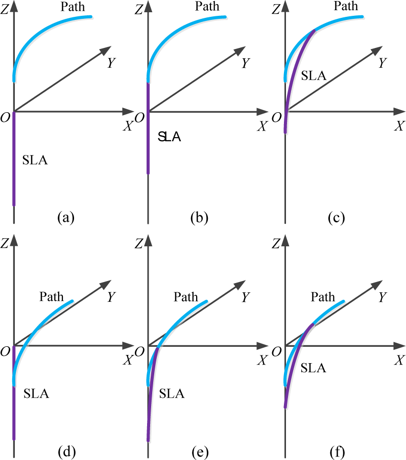
A control flow chart of the AFTIR is shown in Figure 5. The main process is as follows: (1) Conduct the initialization to make the endpoint of SLA reach the origin of the base frame (in this case, the centre of the fuel tank access panel). (2) Confirm the starting point of the path. If it is above the centre of the fuel tank access panel, as in Figure 6(a), then the SLA advances forward in a straight line so that the endpoint reaches the starting point, as in Figure 6(b). If it is below the entry point of the fuel tank, as in Figure 6(d), then the last JS bending action must be controlled in advance. (3) Run the search algorithm based on the varying target points to compute JS variables when the base of the SLA advances one step. (4) Update the pose of the SLA in accordance with the JS variables. If the start point is below the entry point, it can be assumed that the SLA tracks the path from the start point of the path, but starts updating the pose when the end point reaches the origin of the base frame. Figure 6(e) shows the first bending of the SLA, which causes the endpoint to approach the path. (5) Confirm whether the path has been completed or not. If it has been completed, stop the tracking. If not, return to step (3).

Figure 5.

Path tracking flow chart of AFTIR

Figure 6.

Path tracking process

The key issue of the tracking algorithm is to compute the JS variables when the SLA tracks. The search algorithm based on dividing points was proposed here to calculate the JS variables. The ideas of the algorithm are as follows:

4.2.1 Compute the coordinates of dividing points

Each JS of the path is divided into many sections of equal size and the coordinates of the dividing points were computed in frame {B₀}.

Assuming that the length of a JS is L and that the step of the telescopic mechanism is s, then after completing the tracking of one segment of the path, the number of steps that the telescopic mechanism must perform is given as follows:

$w=\frac{L}{s}$

(6) Each segment of the path is divided into w copies, and the coordinates of the dividing points in the frame of the corresponding segment were obtained. Then the coordinates relative to {B₀} can be computed using a homogeneous transformation.

4.2.2 Solve the rotation angle of the end segment of the SLA

When the telescopic mechanism moves one step, the corresponding dividing point is considered the target point, which the endpoint of the SLA should reach. A plane is defined by the dividing point and Z axis attached to the end segment of the SLA. In this way, the rotation angle φ _{R N} , the angle between the x axis and the plane, can be computed.

4.2.3 Solve the bending angle of the end segment of SLA

A numerical method is proposed here to solve the bending angle θ _{R N} as follows: The bending angle is ergodic in accordance with a certain step and the coordinates of the end point of the SLA are obtained each time. Then the distance from the endpoint to the path can be calculated and the bending angle corresponding to the minimum distance can be selected.

The JS variables are recorded at the end of the SLA segment during each step. The JS variables correspond to the path location. The JS variables are the same as those for a corresponding JS when the endpoint of that other JS reaches the same position as the terminal JS. The joint variables of the terminal JS must be computed, but the joint variables of other JS can be obtained directly from the recorded data. In this way, the amount of calculation required does not increase as the number of SLA segments increases. This process also involves low computational complexity and a simple operation.

4.3 Implementation of the tracking algorithm

The tracking algorithm is implemented as follows.

4.3.1 Compute the coordinates of the dividing points in frame {B

₀}

The frame of path JS is {Bg}(g=0,1,2,…,n). Path JS variables of m-th path JS are (θ _{p m} , φ _{p m} )(m = 1, 2, 3, …, n).

The k-th point of the m-th path segment C_{m, k}, as shown in Figure 7, and the bending angle corresponding to this point is θ _{C m,k} , can be expressed as follows:

${\theta }_{C_{m,k}}=\frac{k}{w}{\theta }_{p_m}$

(7) In the path frame {B_m-1}, the coordinate of the point C_{m, k} is given by (8).

${\hspace{0.17em}}^{Bm-1}P{}_{C_{m,k}}=\left(\begin{array}{c}\frac{L}{{\theta }_{p_m}}\cos {\phi }_{p_m}(1-\cos {\theta }_{C_{m,k}})\\ \frac{L}{{\theta }_{p_m}}\sin {\phi }_{p_m}(1-\cos {\theta }_{C_{m,k}})\\ \frac{L}{{\theta }_{p_m}}\sin {\theta }_{C_{m,k}}\end{array}\right)$

(8)

Figure 7.

Division of the path

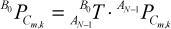
The conversion relationship between the frames of the path segments is similar to that shown in section III. The homogeneous transformation matrix ${\hspace{0.17em}}_{B_{m-1}}^{\hspace{0.17em}\hspace{0.17em}\hspace{0.17em}\hspace{0.17em}\hspace{0.17em}{B}_0}T$ is obtained from frame {B_m-1} to {B₀}. Then the dividing point C_{m, k} coordinate relative to frame {B₀} can be written as follows:

${\hspace{0.17em}}^{B0}P{}_{C_{m,k}}={\hspace{0.17em}}_{Bm-1}^{B0}T\cdot {\hspace{0.17em}}^{Bm-1}P{}_{C_{m,k}}$

(9)

4.3.2 Solve the rotation angle of the terminal segment of SLA

In frame {A_N-1}, attached to the N-th segment of SLA, the plane is determined by C_{m, k} and the Z _{A N-1} axis. Moreover, the path dividing point C_{m, k} is considered to be the target point. The N-th segment of the SLA is on this plane, and the angle between the plane and the X _{A N-1} axis is the rotation angle φ _{R N} , as shown in Figure 8. If the coordinate of the point C_{m, k} is known in frame {A_N-1}, then the value of φ _{R N} can be determined easily.

Figure 8.

Solve the rotation angle of the terminal segment of SLA

The homogeneous transformation matrix from frame {A_N-1} to {B₀} is given as follows:

${\hspace{0.17em}}_{A_{N-1}}^{\hspace{0.17em}\hspace{0.17em}\hspace{0.17em}\hspace{0.17em}\hspace{0.17em}{B}_0}T={\hspace{0.17em}}_{A_1}^{B_0}T\cdot {\hspace{0.17em}}_{A_2}^{A_1}T\cdot {\hspace{0.17em}}_{A_3}^{A_2}T\cdots {\hspace{0.17em}}_{A_{N-1}}^{A_{N-2}}T$

(10) Therefore,

${\hspace{0.17em}}^{B0}{P}_{C_{m,k}}={\hspace{0.17em}}_{AN-1}^{B0}T\cdot {\hspace{0.17em}}^{AN-1}{P}_{C^{m,k}}$

(11) So,

$\begin{array}{l}{\hspace{0.17em}}^{A_{N-1}}{P}_{C_{m,k}}=({\hspace{0.17em}}_{A_{N-1}}^{\hspace{0.17em}\hspace{0.17em}\hspace{0.17em}\hspace{0.17em}\hspace{0.17em}\hspace{0.17em}{B}_0}T\cdot {\hspace{0.17em}}^{B_0}{P}_{C_{m,k}})\hfill \\ ={({\hspace{0.17em}}_{A_{N-1}}^{\hspace{0.17em}\hspace{0.17em}\hspace{0.17em}\hspace{0.17em}\hspace{0.17em}\hspace{0.17em}{B}_0}T)}^{-1}\cdot {\hspace{0.17em}}_{B_{m-1}}^{\hspace{0.17em}\hspace{0.17em}\hspace{0.17em}\hspace{0.17em}\hspace{0.17em}\hspace{0.17em}{B}_0}T\cdot P_{C_{m,k}}\hfill \end{array}$

(12) ^{A _N-1} P _{C m,k} can be obtained in terms of formulas (8), (10), and (12). Based on the geometric relationship, φ _{R N} can also be determined easily, as in equation (13).

$tan{\phi }_{R_N}=\frac{{\hspace{0.17em}}^{A_{N-1}}{y}_{C_{m,k}}}{{\hspace{0.17em}}^{A_{N-1}}{x}_{C_{m,k}}}$

(13)

${\phi }_{R_N}=arctan\frac{{\hspace{0.17em}}^{A_{N-1}}{y}_{C_{m,k}}}{{\hspace{0.17em}}^{A_{N-1}}{x}_{C_{m,k}}}+b\pi (b=0,1,2\cdots )$

(14) The rotation angle φ _{R N} ∈ [0, 2π), according to the projection points in different quadrants, for the value of b is shown in Table 1.

Table 1.

Value of b

Position of projection point	Value of b
First quadrant	0
Second quadrant	1
Third quadrant	1
Fourth quadrant	2

4.3.3 Solve the bending angle of the terminal segment of SLA

The numerical method can be used to solve the bending angle of the terminal segment. The concrete steps are as follows:

(I) Compute the coordinates of the end point of the SLA

The bending angle θ _{R N} remains in the interval [0, π]. During the computing process, θ _{R N} is in the denominator as in equation (2), so it is necessary to select a number close to zero as θ _{R N} =10^-5 instead of θ _{R N} =0. Assuming the angle step is Δθ, then after i steps, the bending angle of the terminal segment of the SLA is given as follows:

${\theta }_{R_{Ni}}=\{\begin{array}{cc}{10}^{-5}& i=0\\ i\cdot \mathrm{\Delta }\theta & i=1,2,3\cdot \cdot \cdot \end{array}$

(15) The coordinate of the endpoint Q_i is $({}^{A_{N-1}}x{}_{Q_i},{}^{A_{N-1}}y{}_{Q_i},{}^{A_{N-1}}z{}_{Q_i})$ , represented by formula (16).

$\left(\begin{array}{l}{\hspace{0.17em}}^{A_{N-1}}{x}_{Q_i}\hfill \\ {\hspace{0.17em}}^{A_{N-1}}{y}_{Q_i}\hfill \\ {\hspace{0.17em}}^{A_{N-1}}{z}_{Q_i}\hfill \end{array}\right)=\left(\begin{array}{c}\frac{L}{{\theta }_{R_N{}_i}}\cos {\phi }_{R_N}(1-\cos {\theta }_{R_N{}_i})\\ \frac{L}{{\theta }_{R_N{}_i}}\sin {\phi }_{R_N}(1-\cos {\theta }_{R_N{}_i})\\ \frac{L}{{\theta }_{R_N{}_i}}\sin {\theta }_{R_N{}_i}\end{array}\right)$

(16) (II) Determine the bending angle based on the distance from the end point of the SLA to the path

When performing process (I), there exists a distance from Q_i to the path for each θ _RNi . The endpoint of the SLA should be as close to the path as possible. The minimum distance can be used to choose θ _RNi as an evaluation standard. Because the path is a special kind of curve, it can be difficult to determine the distance between the endpoint and the path. For this reason, a numerical method is used to determine the distance. When tracking the m-th segment of path, the distances d_ik (k = 1, 2, 3, …, w) from the end point of SLA Q_i to all the dividing points in the m-th segment of the path after the i-th step can be calculated, as shown in Figure 9. Then the minimum can be selected as the approximate value of the distance d_i.

$d_i=\min d_{ik}\begin{array}{cc}& \end{array}k=1,2,3,\cdot \cdot \cdot ,w$

(17) Finally, the minimum distance in d _i (i = 0, 1, 2, 3, …) can be determined, and it can be assumed that i=t in this case. Then the bending angle can be resolved as follows:

${\theta }_{R_N}=\{\begin{array}{c}{10}^{-5},t=0\\ t\cdot \mathrm{\Delta }\theta ,t=1,2,3\cdot \cdot \cdot \end{array}$

(18)

Figure 9.

Calculation of the distance from Q_i to the path divided point C_{m, k}

5. Path tracking simulation for the AFTIR

Several evaluation indexes for the path tracking performance are proposed in order to better evaluate the effects of the algorithm. These are maximum error, average error, response time, and control accuracy.

5.1 Evaluation indexes of the path tracking performance

5.1.1 Maximum error

The maximum error represents the maximum deviation between the segment of the SLA and the path when the SLA of the AFTIR tracks the path. Because only the JS variables need to be solved for the terminal segment of the SLA in the tracking of the path and the other segment repeats the same motions in terms of the motion parameters of the terminal segment, the maximum error can be used to compute the maximum distance between the terminal segment and the path for each step. The maximum value of these maximum distances is called the maximum error.

The maximum error e_max is given as follows:

$e_{\max }=\max d_{\max t}\begin{array}{ccc}& t=1\cdots nw& \end{array}$

(19) Here, d_maxt represents the maximum distance between the terminal segment and the path at the t-th step.

5.1.2 Average error

The average error is the average of all the maximum distances between the terminal segment of the SLA and the path. The average error, ē, can then be set as follows:

$\bar{e}=\frac{{\displaystyle \sum _{t=1}^{nw}{d}_{\max t}}}{nw}$

(20)

5.1.3 Response time

The response time refers to the time required to calculate the JS variables for each iteration. It can be used to express the rapidity of the tracking algorithm.

5.1.4 Tracking accuracy

The tracking accuracy is the distance between the endpoint of the SLA and the endpoint of the path after the tracking is complete. The path is generated by a path planning algorithm based on a given target point. It is the distance from the endpoint of the SLA to the target point. The accuracy of the tracking process can be used to express the accuracy with which the robot reaches the target point.

5.2 Simulation and analysis

Simulations were implemented using MATLAB. The number of segments and the JS variables of each segment were provided after the path planning.

The length L of each JS is 50 cm, and the step values of the base is 1 cm. Table 2 shows the experimental data for a single JS path tracking. From the table, the maximum error and the average error increased gradually as the bending angle of JS increased, and the response time and tracking accuracy fluctuated slightly. However, all these indexes meet the system requirements.

Table 2.

Single JS tracking

Bending angle of Path JS (°)	Maximum error (cm)	Average error (cm)	Response time (ms)	Control accuracy (mm)
30	1.18	0.69	8.92	0.26
45	1.87	1.06	8.86	0.002
60	2.51	1.45	8.71	0.25
75	3.22	1.84	8.80	0.25
90	3.86	2.25	9.02	0.002
105	4.82	2.72	9.16	0.24
120	5.82	3.23	9.19	0.23

The tracking experiment of the planar path with three segments, of which all the rotation angles are 0°, is given in Table 3. Table 4 shows the experimental results of tracking three segment space paths, and the rotation angles of the three segments are different.

Table 3.

Planar path tracking of three segments

Bending angle of path JS (°) θ1 θ2 θ3			Maximum error (cm)	Average error (cm)	Response time (ms)	Control accuracy (mm)
10	30	30	0.60	0.29	23.02	0.40
30	0	0	3.34	1.54	23.02	0.31
30	30	30	1.73	0.99	23.02	0.26
30	60	90	1.51	0.77	23.67	0.70
60	20	45	6.16	2.79	23.13	0.17
90	10	30	9.16	4.23	23.38	0.34

Table 4.

Spatial path tracking of three segments

JS variables of path (°) θ1 φ1 θ2 φ2 θ3 φ3						Maximum error (cm)	Average error (cm)	Response time (ms)	Control accuracy (mm)
30	0	0	0	0	0	3.34	1.53	27.12	0.31
30	0	50	120	75	150	4.61	2.08	27.07	0.11
30	30	60	90	0	0	4.58	1.75	26.64	0.39
45	30	90	120	60	180	7.50	3.08	27.30	0.24
60	80	80	130	15	60	5.54	2.63	27.02	0.17
90	130	10	60	30	0	8.91	4.15	26.95	0.11
100	130	30	90	10	60	8.90	4.36	26.80	0.47

Experimental data show the following: For different paths, the maximum error and the average error are much smaller than the length of JS, indicating that the tracking algorithm was effective. The short response time shows that the algorithm worked rapidly, and the small changes in time confirmed the high stability in the same number of path segments. The value of the control accuracy is very small. The target point deviation is small, indicating that the algorithm was highly accurate.

A prototype was built to validate the proposed tracking algorithm, as shown in Figure 2. A practical experiment was performed. It involved tracking the path with three coplanar segments based on the first group of data in Table 3. As shown in Figure 10, the SLA is able to track the path well. Figure 11 shows a simulation of tracking the path with three coplanar segments, and the experimental data corresponded to the sixth group of data shown in Table 3. Figures 11(a), (b), and (c) illustrate the processes of tracking the first, second, and third segments of the path. During the tracking of the path, the endpoints of each JS of the SLA corresponding to the segments of the path remained close to the path. The SLA remained coincident to the path after completing the tracking, as shown in Figure 11(d). Figure 12 shows the error curve of the tracking of a path with three coplanar segments. The circles represent the maximum distance d_maxt from SLA to the path every step and a straight line stands for the average error e̅. The space path tracking of three segments is shown in Figure 13, and the JS variables come from the second group of data in Table 4. The tracking process is given in Figure 13(a), (b), (c), (d), and each end point of JS is on the path. Figure 13(e) shows the tracking trajectory throughout the whole process. The SLA can track along the path.

Figure 10.

Planar path tracking of three segments. (a) Initialization status. (b) Tracking of the first segment of the planar path. (c) Tracking of the second segment of the planar path. (d) Tracking of the third segment of the planar path. (e) Completion of the tracking of the planar path.

Figure 11.

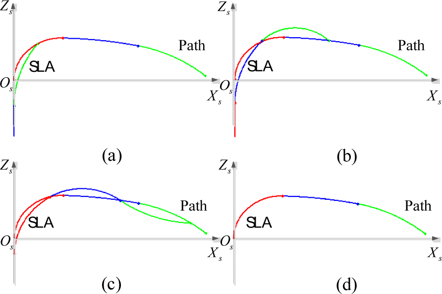
Planar path tracking of three segments. (a) Tracking of the first segment of the planar path. (b) Tracking of the second segment of the planar path. (c) Tracking of the third segment of the planar path. (d) Completion of the tracking of the planar path.

Figure 12.

Error curve of tracking three coplanar segments

Figure 13.

Tracking of the paths of the three segments.

6. Conclusion

In the present paper, a path-tracking algorithm is proposed for the purpose of tracking the planned path and reaching the target for the AFTIR during the process of conducting maintenance on an aircraft fuel tank.

The structural characteristics of the AFTIR are analysed, and kinematic models are established. The proposed algorithm relies on the application of kinematics. The search algorithm, which is based on dividing points, can be used to track the planned path, and a numerical method is used to compute the JS variables. Then by updating the pose, the tracking of the path can be completed. Indexes suitable for evaluating the performance of the path-tracking process have been proposed. Planar and space path tracking experiments were implemented. Experimental results have shown that the tracking algorithm is stable and effective and can be used to carry out the tracking of any given spatial path.