
Abstract
The detection of lane boundaries on suburban streets using images obtained from video constitutes a challenging task. This is mainly due to the difficulties associated with estimating the complex geometric structure of lane boundaries, the quality of lane markings as a result of wear, occlusions by traffic, and shadows caused by road-side trees and structures. Most of the existing techniques for lane boundary detection employ a single visual cue and will only work under certain conditions and where there are clear lane markings. Also, better results are achieved when there are no other on-road objects present. This paper extends our previous work and discusses a novel lane boundary detection algorithm specifically addressing the abovementioned issues through the integration of two visual cues. The first visual cue is based on stripe-like features found on lane lines extracted using a two-dimensional symmetric Gabor filter. The second visual cue is based on a texture characteristic determined using the entropy measure of the predefined neighbourhood around a lane boundary line. The visual cues are then integrated using a rule-based classifier which incorporates a modified sequential covering algorithm to improve robustness. To separate lane boundary lines from other similar features, a road mask is generated using road chromaticity values estimated from CIE L*a*b* colour transformation. Extraneous points around lane boundary lines are then removed by an outlier removal procedure based on studentized residuals. The lane boundary lines are then modelled with Bezier spline curves. To validate the algorithm, extensive experimental evaluation was carried out on suburban streets and the results are presented.
Introduction
Worldwide, a large number of lives are lost each year due to vehicle accidents. In recent years there has been increasing interest in traffic safety systems for reducing vehicle accidents. There are many computer vision-based applications involved in traffic safety systems such as collision avoidance, lane departure warning, and the development of autonomous guided vehicles (AGV) for navigating unstructured environments. The Defense Advanced Research Projects Agency (DARPA) Urban Challenge has generated significant research interest in developing safer autonomous driving systems.
In order to achieve the ultimate goal of autonomous driving in unstructured environments, adequate real-time analysis of the road scene is required (Shang et al. 2013). One important component is the detection of lane boundary lines, and this has received considerable attention in recent years. Lane detection is the problem of identifying road lane boundaries without a priori knowledge of the road's geometry. A number of image-based lane detection algorithms have emerged from autonomous ground vehicle research (Prochazka 2013). Most of the early systems focused on well-paved and structured roads and used a single visual cue such as colour, edge or texture. An automatic lane detection system should cater for both straight and curved lane boundaries, and a wide range of boundary markings including single, double or broken lines, and pavement edges.
Systems based on single cues are more prone to errors because they rely solely on the information provided by the cue. Errors correspond to risk to on-road objects as well as to the autonomous vehicle itself. Feature extraction methods rely on a single visual cue. Such information however, may not always be available. This limitation can be overcome by fusing features from multiple visual cues. In the research by Nilsback et al. (2004), a linear combination of margin-based classifiers for cue integration was proposed. In the method proposed by Birchfield (1998), gradient and colour cues were used for fusion in object tracking. The work proposed by Taylor et al. 2003 fuses colour, edge and texture cues within a Kalman filter framework.
To support real-world application, lane boundary detection algorithms should be able to:
operate subject to shadows caused by road-side trees, buildings, etc.; operate subject to process painted or unpainted road lane lines; handle curved as well as straight roads; and identify lane boundaries on either side of the road.
In this paper a novel lane boundary detection algorithm is introduced. The algorithm integrates multiple visual cues to overcome errors, leading to more robust lane detection. The approach employs supervised learning of road surface chromaticity values, and entropy analysis of image patches containing the road boundary line (Shannon 1948; Gonzalez et al. 2006).
The main contributions of this work are: (a) the use of the CIE L*a*b* colour space and the build-up of a bi-variate Gaussian model, (b) the symmetric Gabor filter for lane extraction, (c) matching entropy values on lane boundaries, and (d) the rule-based classifier for multi-cue integration. This paper is an extension of our earlier work (Lanka et al. 2010).
A large amount of research has effectively addressed the lane detection problem for highway driving. Suburban roads, however, present a very different situation. Highways typically consist of straight roads with multiple lanes and clearly identifiable surfaces, whereas on suburban streets these are uncommon (Wang et al. 2002; Kluge 1994; Aly 2008). Kong et al. (2009) proposed the use of geometric features like vanishing points and textural orientations associated with the straight part of the road for segmenting the road area. In the works by Kluge (1994) and Kreucher and Lakshmanan (1999), a number of geometric models were used to focus on the shape of the road lanes.
For structured and unstructured roads, Alon et al. (2006) combined geometric projection with the Adaboost algorithm to find the drivable road area. The approach however requires a large training set of different road areas in order to train the classifier. Lookingbill et al. (2007) proposed a reverse optical flow technique to adaptively segment the road area. Optical flow, however, varies due to the unavoidable motion of the vehicle, and the method is not robust when other objects such as vehicles, pedestrians, etc., are on the road. When driving on suburban roads, occlusions and poor-quality road markings (resulting from wear) will produce erroneous results. Under such conditions, in order to achieve more accurate and robust classification of the road area, more information is required. The road behaviour can be better approximated by using a statistical model which describes the colour of the road surface based on a training set of images (Goecke et al. 2007). Consequently, algorithms which learn using a visual model and then score the visual field based on that model have proven successful in road detection.
Sensors such as laser and radar have been used for capturing information regarding the road area. Video devices, however, are thought to obtain more information than other types of sensors. Recent research combines laser range finder data with a model of road appearance in RGB colour space using a mixture of Gaussians (Dahlkamp et al. 2006). Goecke et al. (2007) built up a Gaussian model for each pixel of the entire training set by accumulating only the hue and saturation from the HSI colour space. Lipski et al. (2008) proposed a multi-camera lane detection algorithm which uses the HSV colour space. The watershed algorithm is widely used for road segmentation. In the work by Beucher and Bilodeau (1990 and 1994)), who were involved in the European PROMETHEUS project, road and lane segmentation was achieved using a temporal filter, edge detector and the watershed transform. Yu and Jain (1997) used a multiresolution Hough transform to detect lane boundaries. The work, however, does not discuss how to deal with the detection of broken lines or road edges.
Pomerleau (1997) devised the road following control system ALVINN based on a Multilayer Feedforward Neural Network (MLFFNN). The NAVLAB vehicle was equipped with several video cameras, a scanning laser range finder, a global positioning system (GPS) and sonar sensors. ALVINN uses a fully connected three-layer MLFFNN with colour vision inputs from a video camera. In the research by Broggi and Berte (1995), a system was implemented on a parallel SIMD architecture capable of handling data structures which process data at a rate of 10 frames per second. Birdal and Ercil (2007), proposed a vision based system which uses Canny edge detection, texture analysis and Hough transforms to extract contours.
In the works by Kim (2008 and 2006), a real-time lane detection algorithm based on a classifier was proposed to find lane markings. The author also combined the Random Sample Consensus (RANSAC) method with a particle-filtering-based tracking algorithm using a probabilistic grouping framework. Zhang et al. (2005) proposed an approach based on Support Vector Machines (SVM), Image Morphological Operations and an image captured from a bird's eye view. In the research by He and Chu (2007) the detection of lane boundaries was based on edges and the parallel property of the lane edges in a rectified affine space with the use of vanishing point.
Wang et al. (2004) proposed a model for lane detection and tracking based on a B-Snake. In their work, the lane boundaries on both sides as well the understanding of perspective parallel lines were used as the basis to locate the mid-line of the lane. The initial positions for the B-snake model were determined using the CHEVP (Canny/Hough Estimation of Vanishing Points) algorithm. The method proposed by Maček et al. (2004) uses edge detection and colour image filters to extract information regarding the road environment. The information is then processed within a probabilistic framework using particle filters. Assuming a predefined model of the road, the particles are tested to approximate the best vehicle position. A test module based on Canny edge detection and Hough transforms is also used to increase the accuracy and robustness of the system. The system was tested under various real-world road situations including highway traffic scenes, lane changing, magistral inner-city roads with different ground signs, magistral outer city roads with different shadow conditions and windscreen visibility.
Extracting objects and scenes of interest from visual information is one of the biggest challenges in computer vision. Recent advances in object categorization employ statistical methods and artificial intelligence techniques. Most feature extraction and object classification methods rely on measurements obtained from a single visual cue (Filipovych 2007). While these methods work well on a particular class of features appearing in images, they assume that the specific cue is always available. Psychophysical evidence suggests that natural vision based feature extraction and classification tasks are performed by multiple visual cues which are combined to reduce ambiguity. In this paper, such an approach is proved successful in increasing the robustness of lane detection.
Humans use numerous visual cues to localize and classify objects of interest. In the context of extracting road lanes, such cues can be grouped into three parameters: colour, stripe features (lines or almost straight features) and textural features (entropy measure). In the work presented herein, each visual cue provides partial details about an object of interest, which are then combined to classify the object unambiguously. We assume that the visual cues are conditionally independent.
The following section introduces the system for real-time lane detection based on the integration of multiple visual cues and briefly describes the processes involved. The subsequent sections then discuss in detail the key components of the system. Extensive experimental results are then presented which demonstrate operation for different suburban roads.
System overview
An overview of the system is presented in Figure 1. The vehicle-mounted digital camera was mounted on the front left-hand side of the vehicle. As depicted, the system includes offline (training) and online (real-time) processes. The offline processes relate to the generation of a bivariate Gaussian colour model used to classify the road area. The† CIE L*a*b* colour space is employed and the chromaticity values of the individual pixels (a* and b* components) of 50 road surface images are trained with a bivariate Gaussian model using expectation maximization. A training set of as few as 50 images can be used to generate the colour model, which determines the Mahalanobis distance for images as used in the online process. This is discussed in more detail in Section 4.2.

Overview of the system, which includes both offline and online processes
The online processes provide real-time lane detection. After the model is generated, it is used to score the pixels of the first cue based on the Mahalanobis distance. This does not guarantee that all of the road area pixels will be scored as road. Morphological operations are then used to remove unwanted blobs and to isolate the road area as a single connected region. This region acts as an arbitrary region of interest for extracting the edge features from the road area using the asymmetric Gabor filter. For the second cue, the grey entropy (information theory) of image patches is compared to a threshold to isolate the areas containing the road lane boundaries. The two image cues are then integrated using the logical AND operator, to clearly extract the road boundary lines.
The centre points of the blobs are then determined and initial de-noising is achieved through morphological operations followed by the filtering-out of outliers using statistical methods. The road boundary is then estimated by connecting the candidate points with a third degree Bezier spline.
This paper focuses on real-time lane detection using cues as obtained from visual information from a camera mounted on the front left-hand side of the vehicle. This lane detection information could be combined with vehicle kinematic and dynamic models and algorithms to achieve autonomous driving.
In the following section, the extraction of specific features associated with each of the visual cues is described.
Quadrature filters are commonly used for local orientation estimation. A quadrature filter is a complex function whose real part is related to the imaginary part by a Hilbert transform.
A quadrature filter can be represented as follows (in this case the so-called Gabor function):

The Gabor filter is the best-known quadrature filter pair. The real part of the Gabor function is even and sensitive to oriented lines or bar-like features, while the imaginary part is odd and sensitive to oriented edges.
In this research an image is captured from the video device and then filtered by a two-dimensional Gabor filter to extract ridge features. The road lanes in the image appear as bright lines or stripes (with a particular orientation) on a dark background. In terms of greyscale gradient, a line or stripe appears as a sequence of positive gradient (from black to white), followed by a negative gradient (from white to black) of equal or nearly equal magnitude. Edge detection methods such as Roberts, Sobel and gradient-based can also be used to identify a lane line. Most of the time, however, these methods fail to detect ridges or bar-like features and cannot discriminate the lane line or bar features from other edge features. The symmetric Gabor filters react strongly to bar or lane line features which agree with the particular filter parameters.
A number of works have used banks of Gabor filters to extract local image features (Clark et al. 1987; Fogel and Sagi 1989; Tan 1995; Bovik 1991).
To obtain a Gabor feature image f(x, y), an input image I(x, y)for ∀(x, y) ∊ Ω, where Ω can be defined for the set of image points, is convolved with a two-dimensional Gabor filter defined as g(x, y)for ∀(x, y) ∊ Ω (Grigorescu et al. 2002). This can represented as

where the centre of the receptive field Pc(ξ, η) has the same domain Ω.
In our work the following Gabor function is used for extracting line or stripe features (Petkov 1995):

where
The parameter σ determines the linear size of the receptive field. Suppose a response of a cell for a light source is in position Ps(x s , ys). For practical situations, this can then be neglected if |dist(P s − P c )| > 2σ. This effect on cells can be successfully incorporated in the filter used (in this case the Gabor filter) by incorporating the Gaussian factor e−(x′2+γy′2)/2σ2.
The eccentricity of the receptive field ellipse is called the spatial aspect ratio γ. Based on biological research γ is normally selected in the range 0.23 ≤ γ ≤0.92. The angle parameter θ∊ [0, π) specifies the orientation of the normal to the parallel stripes of the Gabor function. The parameter λ is the wavelength of the harmonic factor cos(2π(

Normally this value varies within the small range of 0.4–0.9. The bandwidth value is a real positive number with its default value set at 1. The relationship between σ and λ can be expressed as σ = 0.56λ (as set for our research). The parameter φ ∊ (−π, π], is the phase offset of harmonic factor cos(2;π(
In our work, the best results for road lane detection were achieved using the following parameter values: γ = 0.16, θ = 0, φ = 0 and σ = 5.6 (λ = 10). Figure 2 depicts the schematic diagram and image representation of the Gabor filter for these parameters.

Gabor filter kernel with the chosen parameter set
Figure 3 depicts road image results using the Gabor filter for the chosen parameter set. Figure 3 (a) shows the filtering of a road image with straight lane markings, (b) for a road with left curve markings, and (c) for a road with right curve markings. Figure 3 (d) shows the filter output in the presence of an on road object.

Example scenes demonstrating the output of the Gabor filter
As demonstrated by the results in Figure 3 it is evident that the chosen parameter set for the Gabor filter is robust for different scene variations.
This section discusses the extraction of the road area from the obtained images. This is achieved using a statistical model of the road surface colour built using a set of road surface images. The basic visual model of the road area appearance is a bivariate Gaussian model in the a* and b* space of the CIE L*a*b* colour space. L* is the luminosity and a* and b* are the hue and saturation components specified along the green-red and blue-yellow axes, respectively.
The RGB colour space is a linear colour space and has been used in many algorithms. Using the RGB colour space, difference is calculated as Euclidean distances and thus less computational power is required. The RGB colour space however disregards important information relating to colour complexity.
The CIE L*a*b* colour space is a perceptually uniform colour space designed based on human vision. Using the CIE L*a*b* colour space a constant Euclidean distance represents a fixed perceptual distance. It has been proven that the quality of colour-based modelling algorithms can be substantially improved by using such perceptually uniform colour spaces.
Sections 8.2–8.4 discuss our evaluation of the CIE L*a*b*, CIE L*u*v*, YCbCr and HSV colour spaces for the bivariate Gaussian model. The results demonstrate that the best performance was achieved using the CIE L*a*b* colour space.
Using this colour model, a training set with as few as 50 images provided good experimental results.
Colour information was first captured as an RGB image and then transformed to the CIE L*a*b* colour space. L* was then separated from the chromaticity components. Once the model was built, the region of interest of the road area was converted to CIE L*a*b* colour space and the a* and b* values were extracted. The a* and b* colour values were then used to assign a score based on the Mahalanobis distance. The values (L*, a*, b*) are calculated from the (X, Y, Z)position of the given light stimulus and refer to the specified reference white point.
Parameters of the bivariate Gaussian model
The CIE L*a*b* colour space can be used to make predictions for distinguishing colours in real-world conditions. In most daytime situations, colour discrimination can be based on the two colour values of L*, a* and b*. The perceived lightness of the road surface (illuminated by sun light) is not a reliable visual cue for identification. This is because the road luminance for a given position changes considerably as the viewing angle changes. This occurs because our camera is mounted on a moving vehicle. Research has demonstrated that despite varying luminance conditions, consistency of the chromatic aspects of colour can be maintained as primarily reflected in a* and b* (Simmons et al. 1989). We therefore suggest that distances based on a* and b* should give the best prediction of colour discrimination, and these are used to build the bivariate Gaussian model for road appearance, defined as
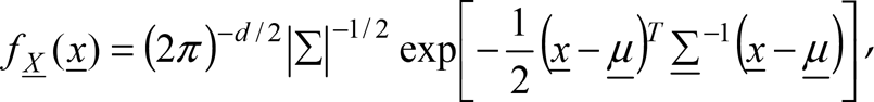
where d = 2,
Initially, a training set H = {

which is the sample mean, and the unbiased estimator of the covariance matrix

After generating the colour model, it is used to classify the road area. The colour model is in the form of a bivariate Gaussian distribution. The Mahalanobis distance from individual pixels to the mean of the learned Gaussian model was used to assign a score to it. The Mahalanobis distance d is defined as

As discussed earlier, the approach presented in this paper uses two visual cues for lane detection. The visual cue with blob features of the road area is insufficient for accurate lane detection alone. The second visual cue employed in this work uses the randomness of the average information content of an image patch.
This research employs a first-order estimate of the entropy measure with the assumption that the image was generated by an imaginary 8-bit grey level source which sequentially emits statistically independent pixels under a predefined probabilistic law.
a*, b* distribution of the bivariate Gaussian model
One method for estimating the probabilistic law for information estimation is to construct a discrete information source based on the relative frequency of the grey levels of a particular image. That is, the grey level distribution of several image patches containing the road lane markings can be interpreted as samples of the behaviour of the grey level or pixels that are generated. This is so because the observed images are the only available indicators of the behaviour of pixel (symbol) probabilities. It is reasonable to use grey level histograms (probability distribution function) to estimate the probabilistic law governing the information source.

Image set showing the classification of the road area using the CIE L*a*b* colour space
Let us assume that a discrete information source generates a random sequence of symbols, where each symbol belongs to a set of distinct possible symbols defined as the source alphabet A.
This can be represented by A = {a1, a2, …, aJ}, where each aj is a symbol. If the probability of generation of symbol aj by the discrete information source is p(aj), the probabilities of source symbols can be represented by vector
The self-information, or the amount of information generated by the production of a single source symbol aj, is defined by I(aj) = −log b p(aj), where b is the base of the logarithm determining the unit of the information measure. If k source symbols are generated, and if the symbols generated by the discrete source are represented by a random variable X, the average self-information of X or the entropy of the source is denoted by

where X ∊ A.
In this research, random variable X represents the pixel grey value generated for a rectangular image patch where the image patch can be assumed as an imaginary grey level pixel source analogous to a discrete information source in information theory.
Given a particular r th video frame denoted by Xr, a rectangular image patch can be defined by Xr[x − w…x + w, y − w…y + w] where w denotes half of the window size in the x and y directions. The pixel coordinates x,y of the image patches are selected in such a way that pixels of an image patch only need to be used to calculate the Shannon entropy once. The updates would then be defined by x = x + 2w and y = y + 2w.
The matching criteria are then considered for the image patch entropy H(Xr)to be within the range between thlow and thhigh, where thlow and thhigh are the low and upper threshold values, respectively. If thlow ≤ H(Xr) ≤ thhigh, then the image patch is considered to contain a substantial amount of lane features or lane information. If this condition is not met, the image patch is considered to belong to another part of the image.
Suitable values for thlow and thhigh were estimated by analysing the grey image entropy of test image patches containing lane features (Figure 6). If smaller image patches are used, many image areas may be identified as lanes, whereas larger image patches may remove the majority of lane features.

Test image patches of size 20×20 pixels containing lane features used to estimate thlow and thhigh.
Through analysing different image patch sizes, the half window size w = 9 provides a good compromise between the amount of self-information and processing speed. Since the base of the logarithm b = 2 was used, empirical estimates for thlow and thhigh, of 4.0 and 4.7 bits/pixel, respectively, were selected.
Figure 7 shows entropy image results for test road images with the selected lower and upper threshold parameters. The first image pair shows the original and entropy images of a road with straight lane markings; the second pair of a road with left curve markings; the third pair of a road with right curve markings, and the final image pair shows lane markings in the presence of a vehicle object.

Original and corresponding entropy images for a particular luminance level.

Modified Sequential Covering Algorithm (MSCA) for visual cue integration
Visual cue integration
This paper focuses on a lane boundary detection algorithm which integrates two visual cues. In the development of such a multi-cue system, the method by which the individual cues are integrated is a vital consideration.
In this work, the image cues from both the Gabor filter and entropy image analysis are thresholded and morphological operations applied in order to emphasize the candidate lane markings and to remove unwanted objects. As a result, both image cues to be integrated take the form of binary images. The two visual cues are then integrated using a modified rule-based classifier, resulting in a lane image emphasizing lane markings while eliminating most of the unwanted areas within the region of interest.
Modified rule-based classifier
Rule-based classification methodologies offer clarity and simplicity in rule implementation and have been widely used in real-world applications.
Most rule-learning algorithms in rule-based classifiers follow the separate-and-conquer or covering strategies, where rules are learnt one at a time, covering part of the training examples. Such a classification rule can be expressed by
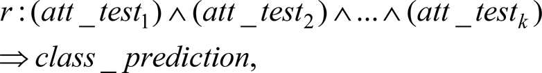
where att_testk is the k th attribute test, which is logically ANDed to the other attribute tests; class_prediction is the class prediction of a test record. The training examples covered by the newly added best rule are separated before subsequent rules are added, i.e., before the remaining training examples are conquered. This concept of extracting best rules directly from data can be found in the well-known Sequential Covering algorithm. In the algorithm, rules are grown in a greedy fashion based on evaluation metrics such as FOIL_Gain or Likelihood_Ratio (Furnkranz and Flach 2003; Han and Kamber 2006).
A rule-based classifier can be represented by R = (r1 ∨ r2 ∨ … ∨ rk), where R is the classifier or rule set, and ri are the classification rules. In this research, we propose a modified sequential covering algorithm to select the best-represented visual cues (with their selected attributes and values), and integrate them to extract the lane markings with high accuracy. The classifier's class prediction relates to whether the pixel represents a lane or not. As such, this is a binary classification process with no conflicting classes. Where necessary a disjunction (logical OR) is then used between the generated rules. Since the rule set does not guarantee exhaustive coverage of every combination of attribute tests, in the case of a failed test, a default rule is used. The default rule is as follows: if c = 1 represents the class prediction or lane class, the class prediction of the default rule is
The modified sequential covering algorithm (MSCA) is described in Algorithm 1. MSCA aims to extract the rule with the maximum vote from the best generated rules each iteration. As with the standard sequential covering algorithm (Han and Kamber 2006) rules are grown in a general-to-specific manner. This is like a beam search, where the initial rule set is set to null, then attributes are gradually appended to the current rule antecedent using the logical conjunct which best improves the rule (determined based on a quality measure).
Suppose the training data set I, consists of a set of images Ij, where j = 1,2, …, n, and each image represents a different state of the road lanes such as straight and curved lanes, and the presence of different objects (e.g., pedestrians and vehicles), for a particular luminance level. Due to different variations of the appearance of lane boundary lines, each image Ij was used separately for rule extraction.
In a manner similar to the standard sequential covering algorithm, the Learn_One_Rule function was used to extract the best set of rules for lane extraction. Attributes considered to find the best rules include Mahalanobis distance-based voting of lane colour, Gabor filter output and grey level entropy. For a particular luminance level the possible values for the entropy attribute were found to have a common range. The other attributes also share this characteristic. The MSCA then selects the set of attribute ranges for the visual cues to best describe the lane boundary lines.
The Learn_Qne_Rule function selects the best attribute test to append the current rule, based on a rule quality measure. The rule quality measure considers whether the attribute test to be appended will result in improving the rule.
The rule quality measure comprises two quality measures, namely FOIL_gain and Likelihood_Ratio. FOIL_gain is based on information gain while Likelihood_Ratio is a statistical-based test. Simple measures such as coverage or accuracy are not reliable measures of rule quality, and FOIL_gain and Likelihood_Ratio were chosen for a better understanding of how rules are selected.
Let p be the number of positive examples and n the number of negative examples, covered by the current rule R. If an attribute test is appended to the current rule R it is represented by

The Likelihood_Ratio quality measure uses a statistical test of significance to determine the correlation between attributes and classes. The Likelihood_Ratio is defined as

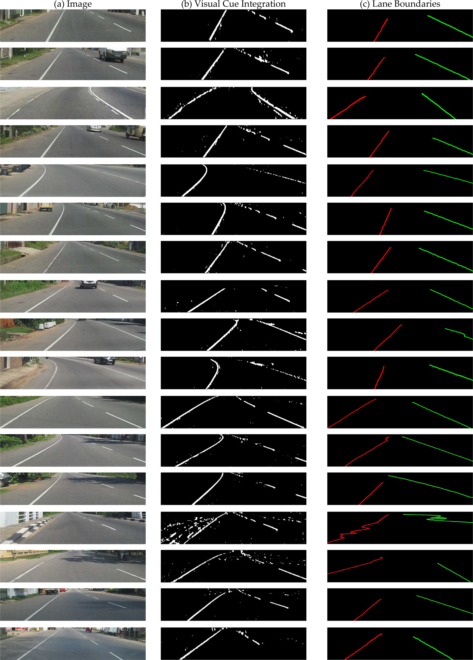
where k is the number of classes, fi is the observed frequency of class i examples covered by the rule, and ei is the expected frequency of a rule which makes random predictions. The Likelihood_Ratio has a chi-square distribution with k − 1 degrees of freedom (Han and Kamber 2006). Figure 8 shows the result of integrating the two visual cues obtained from the MSCA.

Examples of visual cue integration
After the segmentation of road lane boundaries, the left and right lane boundaries need to be separated. Figure 9 shows an example of classifying the road area and separating the lane boundaries.

Extracted source images for further separation of lane boundary lines to left and right
The classification of the road area begins by division into three rectangular regions, where each region can be considered as a connected component. The regions are defined by two horizontal lines dividing the rectangle into three equal sized rectangles, as can be observed in Figure 10. The centroids

where

Division of the road area into rectangular regions and definition of unit vectors for identifying lane boundary points on the left and right sides
The centroids P, R of the first and third rectangular regions are then connected to the centroid of second rectangular region Q, using two straight lines. Normal vectors u, v are then determined for the two lines. As demonstrated by Figure 10 the road area image (of Figure 9 (a)) is then divided into two parts using a horizontal reference line (red colour) passing through the centroid of the second rectangular region.
The image of Figure 9 (b) was used to find the lane boundary points by dividing the image to a number of rectangular regions considered as connected components. The centroids of the connected components were then calculated using moments. The basis for using a much larger number of rectangular regions is to collect an adequate number of points for sufficiently smooth lane boundaries.
At this point, a collection of lane boundary points have been determined, but have not yet been differentiated as belonging to the left or right lane boundaries.
Boundary points above and below the reference line (shown in Figure 10) can be considered as the following sets, respectively:

In order to determine which side of the lane the points in St belong to, the vector dot product between normal vector u, and the vector joining position vector P to each of the position vectors in St, is used. Similarly, to determine which side of the lane the points in Sb belong to, the vector dot product between normal vector v and the vector joining position vector R to each of the position vectors in Sb, is used. If the vector dot product is greater than or equal to zero, the point in either St or Sb belongs to the right-side lane boundary. Otherwise the point belongs to the left lane boundary.
One issue observed in identifying lane points was outliers, which can deform the shape of the lane boundary. Outlier points were filtered out using studentized residuals for the data points of either the left or right lane boundary. Suppose the data points identified for the left lane boundary are Sl = {(xl1, yl1), (xl2, yl2),…, (xlm, ylm)} consisting of m data points. The set of points
The straight line model was used because straight lane boundaries can be easily modelled. Furthermore, curved lane boundaries as seen from the vehicle-mounted camera, appear to be approximately straight. A similar straight line model can also be fitted to data points identified for the right lane boundary Sr = {(xr1, yr1), {xr2, yr2), …, (x rn , y rn )} consisting of n data points.
Residual analysis for outlier detection
Using the straight line regression model, the residuals are defined as

where the Mean Square Error (MSE)

Based on the assumption of a standard normal distribution of residuals, approximately 78% of the studentized residuals were identified to be in the range (−1.2, 1.2), providing a good measure for filtering outliers. Residuals outside of this interval indicate outliers considered as extreme cases. Figure 11 depicts outliers (shown in blue) rejected by the algorithm.

Separating the lane boundary points to left and right
Third-degree Bezier spline curves using Bernstein polynomials were fitted to the data points of the left and right lane boundary points (with outliers removed). Third-degree Bezier splines provide reasonable design flexibility without the increased computation required for higher-order polynomials.

where the k th Bernstein polynomial of degree n is defined as

This section compares the theoretical basis of our system with other similar systems and verifies the accuracy and performance of our system.
Data collection
In this experiment, images were obtained from a digital camera mounted on a moving vehicle. A total of 75 images of 640×480 resolution were collected.
To build the Gaussian model, chromaticity values were collected from sample rectangular areas on the road surface, cropped from 50 of the collected images. The remaining images were used for testing.
The image set comprised a wide variety of conditions common to suburban roads. These include straight and curved roads (with and without on road obstacles, and with clear and worn lane boundaries) as well as lane boundaries subject to interference from the shadows of trees and road-side structures.
Parameter tests for the Gabor filter
To obtain the best parameters for the Gabor filter, an extensive number of parameter evaluations were performed. Figure 12 depicts Gabor filter responses and corresponding kernels for different test parameters.

Gabor filter output for test images and different selected parameters
It is important to observe that a satisfactory amount of lane markings was detected when 0 ≤ σ/λ ≤ 0.6 and 0 ≤ γ ≤ 0.5. Values for σ/λ were determined using equation 4 for bandwidth values 0.5, 1 and 2, where the default value is 1.
To classify the road area, the bivariate Gaussian model was built using several colour spaces, namely the CIE L*a*b*, CIE L*u*v*, YCbCr and HSV colour spaces. Only the chromaticity of these colour spaces, representing hue and saturation, was used. The most important consideration in selecting these colour spaces is the ability to separate the luminance and chromaticity components. Modelling the road area based on colour values helps to distinguish and extract the road area from other similarly shaped objects in an accurate and convenient way.
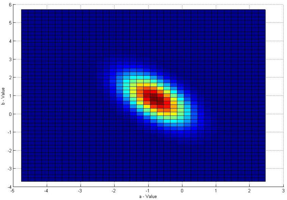
Figure 13 depicts the bivariate Gaussian models based on the chromaticity values of the different colour spaces. Figure 13 (a) shows how a* and b* values are distributed in the bivariate Gaussian model. Figures 13 (b), (c) and (d) show how u* & v*, Cb & Cr, and H & S values are distributed in the bivariate Gaussian model.

Bivariate Gaussian models for chromaticity values of different colour spaces
In order to analyse the effectiveness of the Gaussian fitting, the chi-square plots of the generalized distances (Mahalanobis distances) were used. The plots for the chromaticity values of the CIE L*a*b*, CIE L*u*v*, YCbCr and HSV colour spaces were used to identify the best-fit model. These plots are shown in Figure 14.

Chi-square plot of the generalized distances of the chromaticity values extracted under different colour spaces
According to Johnson and Wichern (2002), if a data set of size of n, with each dimension of p ≥ 2, is of multivariate normality, then squared distances dj2 for j = 1,2, …, n should behave like a chi-square random variable. Figure 14 shows the chi-square plot of the generalized distances of the chromaticity values extracted under the different colour spaces.
Theoretically, for multivariate normality the data set should resemble a model of a straight line passing through the origin with a slope of magnitude 1. In this work, three different objective statistics are used to analyse and select the model which best fits the real data. These statistics are the Akaike Information Criteria (AIC), Bayesian Information Criteria (BIC), and the adjusted coefficient of multiple determination Radj2.
The AIC statistic is defined as

where Lmax is the maximum likelihood achievable by the model, and k is the number of model parameters (Akaike 1974). The best model is the one which minimizes the AIC statistic.
The BIC statistic, or Schwarz Criteria (Schwarz 1978), can be defined as

where N is the number of data points used for fitting. Like the AIC statistic, the best model is the one with the lowest BIC value.
The third statistic Radj2 refers to the amount of variability in the given data set as assessed by a regression model, and varies between 0 and 1 (Montgomery and Runger 2003).

where SSE/(n − p) and SST/(n − 1) are the residual and total mean sums of the square respectively. The model with the maximum Radj2 value indicates the best fit.
The results of fitting the straight line model are summarized in Table 1.
Comparison of AIC, BIC and Radj2 statistics for analysing the best fit
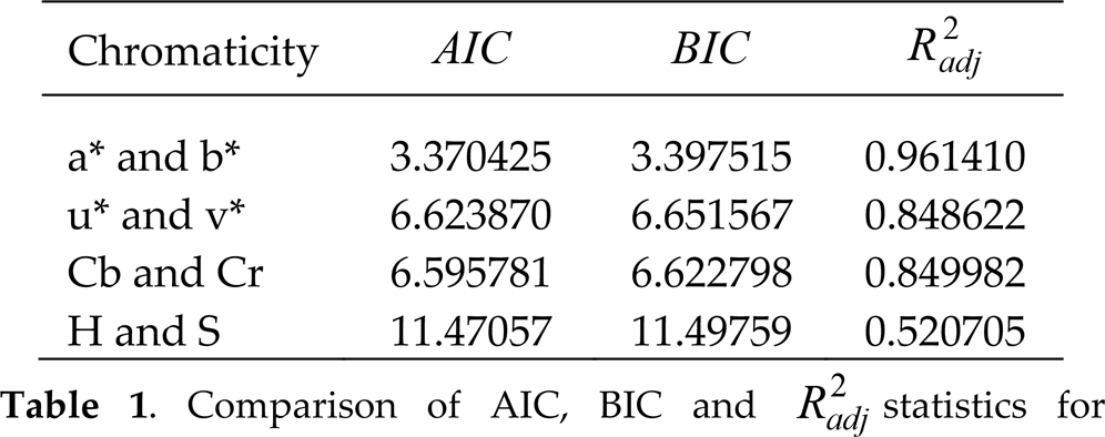
One significant finding is that the model fitted to the a* and b* chromaticity values has the lowest AIC and BIC values, and the highest Radj2 value.
All of the straight line models demonstrate a lack of normality, with a* and b* representing the best of the different chromaticity values. This indicates that the a* and b* chromaticity values have the best bivariate normal fit. This was further evaluated using experimental data.
Figure 15 shows the test results obtained using the different bivariate Gaussian models to classify the road area for different classes of environments, i.e., roads with straight and curved lane boundaries. In addition, tests were performed for detecting lane boundaries subject to on road shadows of road-side trees and other structures. There were instances where shadows appeared on the road. In these cases the CIE L*u*v* and YCbCr colour spaces performed relatively poorly, while CIE L*a*b* provided better results.
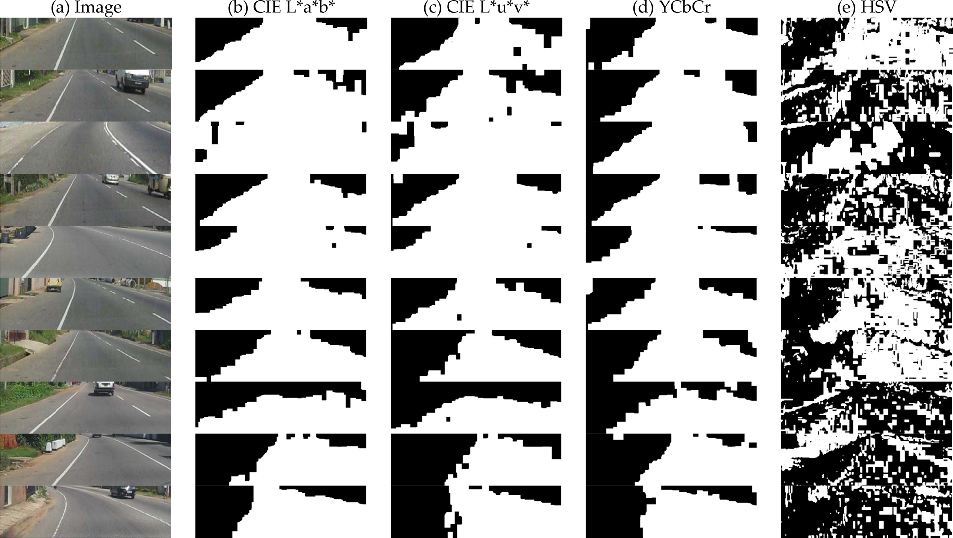
Results using the bivariate Gaussian models for classification of different environments (a) Original image, (b) bivariate Gaussian with a* & b*, (c) bivariate Gaussian with u* & v*, (d) bivariate Gaussian with cb & cr, and (e) bivariate Gaussian with H & S.
The HSV colour model performed poorly in almost all cases. This is supported by Table 1 where the HSV colour space had the highest AIC and BIC values as well as the lowest value for Radj2. The Gaussian models based on u*, v* and Cb, Cr performed classification with similar performance. This is supported by the results of Table 1 and the test results shown in Figure 16. Figure 16 demonstrate results using the bivariate Gaussian models to classify subject to shadow conditions. These results demonstrate the increased robustness of the a* and b* chromaticity values compared with the other colour spaces.

Results using the bivariate Gaussian models to classify subject to shadow conditions. (a) Original image, (b) bivariate Gaussian with a* & b*, (c) bivariate Gaussian with u* & v*, (d) bivariate Gaussian with cb & cr, and (e) bi-variate Gaussian with H & S.
In the experiments, the integration of the different visual cues with the modified rule base classifier was performed. The classifier aims to not only improve the accuracy of detecting lane boundary lines, but to also make the integration process much simpler than traditional integration techniques like the Bayesian method (Filipovych et al. 2007) and hidden Markov model (HMM) (Wei and Piater 2008).
In this section, the implementation of an extension to the rule set to cater for different luminance levels is discussed. Algorithm 2 was used to select the best-voted rules from sets of images with different luminance levels. The average luminance levels were evaluated using the L* component from the search area windows of the road images.

Rule-based classifier for different luminance levels
These average luminance levels are represented by {avg_lum1,…, avg_lum q }, and then for each luminance level the best-voted rule is selected using the MSCA (algorithm 1). An example of selecting the best-voted rule from an image set for particular a luminance level is discussed below.
Table 2 shows the pixel counts for lane boundary lines within a set of images using the most general rule R0. For this initial rule, the attribute set of the rule antecedent is empty, and for a straight-lane road the image covers p0 = 1813 positive examples and n0 = 63467 negative examples.
Pixel counts for lane boundary lines covered by the initial rule R0
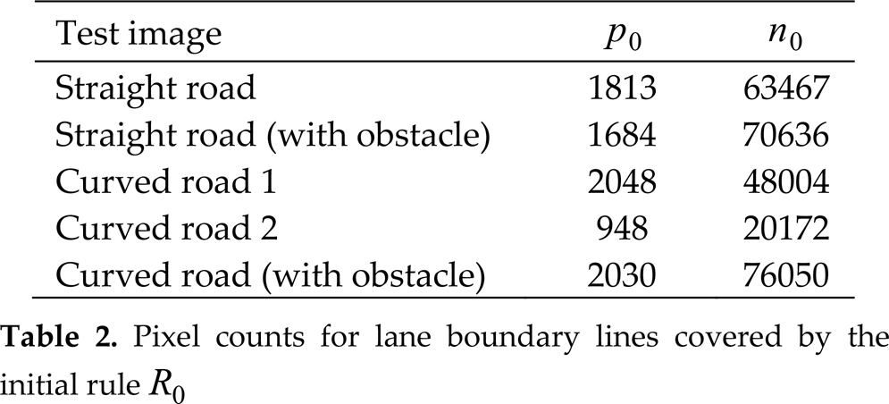
Table 2 shows the number of pixels used for the initial rule taken from five different test images. Using the Learn_One_Rule function of algorithm 1, and by analysing the coverage of positive and negative pixels, the output of the Gabor filter has the maximum rule quality with respect to other attribute value ranges.
The Gabor-based attribute was selected as the first attribute test in conjunction with another attribute. From a predefined set of colour distance and entropy ranges, the Gabor-filtered image was best covered for lane boundary lines by the entropy attribute. The entropy attribute was better than the colour attribute and this can be proven using the FOIL_gain and Likelihood_Ratio quality measures.
This gives our final rule of using attributes Gabor-filtered and entropy images.
The image output from the modified rule classifier is then used to identify the candidate lane boundary points. These points may contain the points representing the real lanes as well as outliers.
Here, outlier detection of these candidate points under different significance levels are compared and evaluated. The test was performed for the categories of straight roads and curved roads (both with and without obstacles). For each category, ten test images were selected and the average detection of outliers was calculated for four different significance levels (99%, 95%, 87% and 78%) based on the studentized residuals discussed in Section 7. The results are presented in Table 2. It can be observed that outlier detection at the 78% significance level (studentized residuals between [−1.2, 1.2]) performed best for each category. The performance achieved was 100% for straight roads, 98.9% for curved roads, 97.8% for straight roads with obstacles, 85.6% for curved roads with obstacles, and 82.4% for straight roads with shadows.
This performance helps in modelling lane boundaries with better accuracy than for other levels of significance. This is especially true for the case of curved roads.
Test results for the detection of lane boundaries within different environments
Over the past few decades, real-time lane detection systems for autonomous vehicles have received significant research interest. Unlike parametric lane-fitting methods based on Hough transforms or other single-cue based approaches, this paper presents a novel method using cues from a symmetric Gabor filter and an entropy image. The cues are combined with a modified rule based classifier to estimate the lane boundaries of unstructured suburban roads. Interestingly, it was observed that, subject to on-road obstacles and shadows, the proposed method provided better results than parametric approaches. The algorithm is capable of extracting lane boundaries from a 640×480 image in less than 90 ms, demonstrating acceptability for real-time operation. The results demonstrate that the proposed lane boundary detection algorithm performs well compared with other lane detection algorithms for a variety of conditions.
Footnotes
10.
The paper presents experimental results for real-time lane boundary detection within different environments. The algorithm uses multiple visual cues to achieve a robust solution. In order to benchmark our solution against other algorithms, future work will involve a much larger experimental data set including much more diverse suburban environments. This will enable comparison with existing single and multi-cue approaches with respect to a variety of criteria including robustness, computational expense and latency.
11.
Waduge Shehan Priyanga Fernando is a lecturer in the Department of Mechanical Engineering, Faculty of Engineering, General Sir John Kotelawala Defence University in Sri Lanka, where he has worked in this position since April 2012. He received his BSc (Eng.) specializing in Computer Science & Engineering from the University of Moratuwa in 2004 and his Master of Philosophy in the Department of Electrical Engineering from the same university in 2011. Prior to joining the faculty, he was a system analyst at the University of Moratuwa from 2007 to March 2012, and an associate system engineer at Data Management Systems (Pvt.) Ltd. (2004–2007). His research interests include Computer Vision, Computer Graphics, Artificial Intelligence, Mathematical Optimization, Localization, Map Building and Navigation of robots. Mr Fernando has co-authored more than ten publications presented at international and local conferences. He is a member of the Sri Lanka Association for the Advancement of Science (SLAAS), a premier organization of scientists in Sri Lanka.
Lanka Udawatta received his BSc (Eng.) in Electrical Engineering from the University of Moratuwa, Sri Lanka, in 1996. He received his MEng and PhD degrees from Saga University, Japan, in 2000 and 2003, respectively. His research interests include Systems Control, Mechatronics, and Artificial Intelligence Applications in Electrical Engineering. Dr Udawatta has co-authored more than 50 publications for peer-reviewed international journals and international conferences, and has also published one book, “Computer Aided Simulations”. Dr Udawatta has served on many technical committees, including for IEEE conferences, journals and transactions.
He is a chartered electrical engineer and a senior member of IEEE. Since 2012 he has been with RAKMC, Higher Colleges of Technology, UAE.
Ben Horan (Member IEEE) received a BEng degree with first-class honours and a PhD degree from Deakin University in 2005 and 2009 respectively. Since 2008 he has been with the School of Engineering, Deakin University, Australia, where he is a Senior Lecturer and Coordinator for the Mechatronics discipline. His current research interests include Haptic-Human Robotic Interaction, Haptic Device Design and Mobile Robotics.
Pubudu N. Pathirana (Senior Member IEEE) was born in 1970 in Matara, Sri Lanka, and was educated at Royal College, Colombo. He received a BEng degree (first-class honours) in electrical engineering, a BSc degree in mathematics in 1996, and a PhD degree in electrical engineering in 2000, all from the University of Western Australia and sponsored by the government of Australia on EMSS and IPRS scholarships, respectively.
He has worked as a postdoctoral Research Fellow at Oxford University, Oxford, UK, a Research Fellow at the School of Electrical Engineering and Telecommunications, University of New South Wales, Sydney, Australia, and a Consultant to the Defence Science and Technology Organization (DSTO), Australia, since 2002. He was a Visiting Associate Professor at Yale University, New Haven, CT, in 2009. Currently, he is an Associate Professor with the School of Engineering, Deakin University, Geelong, Australia, and his research interests include Mobile/Wireless Networks, Autonomous Systems, Signal Processing and Vision-based Systems.
†
CIE – Commission International d'Éclairage