Sage Journals: Discover world-class research

Abstract

Although an autonomous underwater vehicle (AUV) is noted for its good autonomy, concealment and anti-interference ability, errors in its inertial navigation system (INS) inevitably increase over time, leading to positional failure during long-term voyages. Terrain-assisted navigation can help the INS to correct its position. The traditional iterative closest contour point (ICCP) achieves high matching accuracy when the initial position error of the INS is small, but is prone to mismatching when the initial error is large. This study combines ICCP with particle swarm optimization (PSO) to overcome this problem. First, the global optimization ability of PSO is improved by changing the acceleration factor and introducing an artificial bee colony (ABC) onlooker bee greedy search (ABC-ωAPSO). Second, the Euclidean distance of ICCP is replaced by the Mahalanobis distance to abate the influence of system error on the matching accuracy. Finally, the initial position error is reduced by rough matching using the ABC-ωAPSO, which has global optimization capability. Next, fine matching is performed by ICCP. This two-step process resolves the sensitivity problem of ICCP to the initial position error. The experimental results revealed a good matching effect after the double-matching procedure. When the initial INS errors were 0.55′ to the east and 0.55′ to the north, the matching error was reduced to 89.3 m, suggesting that the approach can realize autonomous passive navigation of AUVs.

Keywords

ICCP Mahalanobis distance PSO ABC

Introduction

Autonomous underwater vehicles (AUVs) are being used increasingly in military and commercial applications because of their capability for autonomous navigation. However, location errors are common in long-distance, deep-dive, and all-weather missions; the cumulative errors in the inertial navigation system (INS) can be corrected by terrain-aided navigation (TAN) algorithms, which match the measured topographic distribution characteristics to the background of the terrain data. As the original terrain-database information is contained in the sounding-point location information, the measured terrain-elevation distribution can be obtained from the real-time location information in the background field and employed for aiding the error correction of the inertial navigation.^1–4 The matching algorithm plays a very important role in the TAN system. Iterative closest contour point (ICCP) is one of the most commonly used terrain-matching algorithms, which is advantaged by high precision and easy implementation. Further, ICCP has high matching accuracy when the initial error is small, but it often has poor matching accuracy when the initial error is large.^5–7

ICCP has been improved by many scholars. Liu et al.⁸ proposed a real-time ICCP with an optimized matching sequence length (OMSL-ICCP), which can obtain the current optimal matching sequence length through searching the current measurements to reduce matching error. Wang et al.⁹ replaced the Euclidean distance with the Mahalanobis distance in ICCP to improve the anti-interference ability of the algorithm. Wang et al.¹⁰ proposed a parallel ICCP algorithm, which improves the matching accuracy of ICCP for large initial errors but is computationally time-intensive. Alternatively, Ji et al.¹¹ and Gao et al.¹² applied particle swarm optimization (PSO) and artificial bee colony (ABC) algorithms for INS matching. These algorithms reduce the matching time and improve the matching effect, but their matching accuracy for large initial position errors requires further investigation. Some scholars have combined ICCP with other algorithms in complementary schemes that exploit the different performances of different algorithms. Xu et al.¹³ proposed a new PSO-ICCP that effectively improved the matching accuracy. Yuan et al.¹⁴ combined the matching results of terrain contour matching (TERCOM) and ICCP. The difference between the two matching results was input to a Kalman filter to reduce the matching error. Unfortunately, the speed of matching using this approach is slow. Ding et al.¹⁵ and Zhang et al.¹⁶ both implemented a two-stage, coarse-fine matching algorithm to enhance the matching accuracy. To function effectively, these algorithms necessitate the integration of data from the multi-beam echosounder (MBES), an apparatus that demands both high computational capability and stringent prerequisites.

The traditional ICCP has higher accuracy under small initial position errors, indicating that local searching well converges under this circumstance. However, matching failures often occur under large initial position errors. To enhance the performance of the traditional ICCP for large initial position errors, the INS indicator tracking can be preprocessed by ABC optimization adaptive PSO (ABC-ωAPSO), and then refined by ICCP. The two algorithms achieve effective complementarity; that is, the fast global optimization capability of ABC-ωAPSO complements the local refinement capability of ICCP. The main contents of this research are summarized below.

(1) The Euclidean distance in ICCP is replaced by the Mahalanobis distance as the objective function. The Mahalanobis distance reduces the influence of noise and improves the stability of the algorithm.

(2) To remove the sensitivity of ICCP to the initial position error, the initial position error is first reduced by ABC-ωAPSO. ICCP is then applied for precise matching and the matching accuracy is improved by the quadratic matching strategy.

(3) The acceleration factor of PSO is first improved and a peak greedy search is then introduced to improve the global optimization ability of PSO, and hence the rough-matching effect. The improved PSO for fine matching by ICCP.

(4) The conclusion is obtained through the simulation experiment.

ICCP and improvement

ICCP algorithm

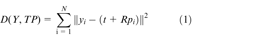
ICCP uses the minimum square of the Euclidean distance as the objective function to obtain the optimal rigid transformation between the measured trajectory and true trajectory, so as to obtain the corrected trajectory. ICCP searches for the point set closest to the indicated location of the INS on the isobath, as shown in Figure 1. In Figure 1, A_i (i = 1, 2 …N) represents the bathymetric measurement point on the real track, where N is the length of the matching sequence; C_i (i = 1, 2 …N) represents the isobath; p_i (i = 1, 2 …N) is the indicated location of INS; y_i (i = 1, 2 …N) is the matching location. ICCP iterates continuously to find T, and T represents the rotation transformation (R) and translation transformation (t) of each iteration; then, the distance-squared function D between the current iterative point set p_i after transformation and the closest point set y_i of p_i on the isobath C_i is minimized, as shown in equation (1). The transformed point set Tp_i of the current iteration point set p_i is taken as the next iteration point set. After several iterations, the set of iterative points satisfying the convergence conditions is taken as the final set of matching points.¹⁷

D (Y, TP) = \sum_{i = 1}^{N} {‖ y_{i} - (t + R p_{i}) ‖}^{2}

(1)

Figure 1.

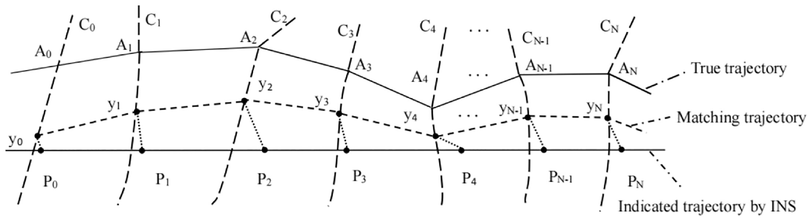
Principle of the ICCP.

According to the ICCP principle, the traditional ICCP has great limitations in application:

(1) If the location indicated by INS greatly differs from the true location, it will lead to mismatch divergence or even mismatching.

(2) ICCP is based on the data reference map, but there are errors in data acquisition and contour drawing.

To overcome these limitations, we improved the traditional ICCP as follows.

Improved ICCP algorithm

ICCP does not consider the influence of depth measurement errors and isobath drawing errors in the algorithm. Hence, the Euclidean distance was replaced by the Mahalanobis distance to abate the influence of errors on the system. Thus, the matching accuracy of ICCP was improved to make the algorithm more practical. The Mahalanobis distance can eliminate the interference of variable correlation.

The Euclidean distance equation (1) is replaced with the Mahalanobis distance equation (2).

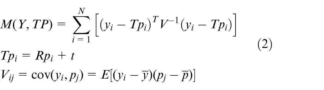
\begin{matrix} M (Y, TP) = \sum_{i = 1}^{N} [{(y_{i} - T p_{i})}^{T} V^{- 1} (y_{i} - T p_{i})] \\ T p_{i} = R p_{i} + t \\ V_{ij} = cov (y_{i}, p_{j}) = E [(y_{i} - \bar{y}) (p_{j} - \bar{p})] \end{matrix}

(2)

where V_ij represents the covariance matrix of the (i,j)th term; $\bar{y}$ and $\bar{p}$ are the mean of the sample. ICCP takes the position with the minimum M value as the optimal position.

ABC-ωAPSO terrain-matching algorithm

In order to reduce the initial position error, it needs to be preprocessed. Because PSO performs fast optimization, it is employed for initial matching. However, the classical PSO is prone to local optimality. To avoid this problem, we apply the improved PSO for rough matching, and then the improved ICCP is used for fine matching.

Improved PSO algorithm

The classical PSO is a random optimization algorithm based on population. The equations of PSO with inertial weight as introduced by Shi and Eherhart are shown in equations (3) and (4).^18,19

\begin{matrix} {v_{i}}_{j} (τ + 1) = ω {v_{i}}_{j} (τ) + φ_{1 j} [gbes t_{j} (τ) - {x_{i}}_{j} (τ)] \\ + φ_{2 j} [pbes t_{ij} (τ) - {x_{i}}_{j} (τ)] \end{matrix}

(3)

{x_{i}}_{j} (τ + 1) = {x_{i}}_{j} (τ) + {v_{i}}_{j} (τ + 1)

(4)

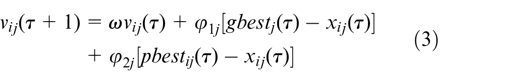
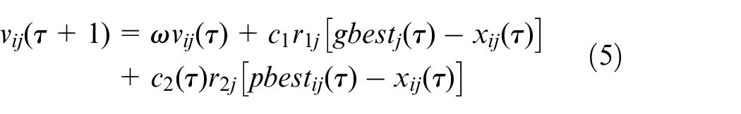
where i represents the total number of particles (i = 1, 2, …., s); j represents the dimensions (j = 1, 2, …., n); $φ_{1 j} (τ) = c_{1} r_{1 j} (τ)$ , $φ_{2 j} (τ) = c_{2} r_{2 j} (τ)$ , where c₁ and c₂ are acceleration factors; $r_{1 j} (τ), r_{2 j} (τ) \in (0, 1)$ are random numbers; ω is the inertial weight; ${x_{i}}_{j} (τ)$ is the location of particle i in the jth dimension at time $τ$ ; ${v_{i}}_{j} (τ)$ is the velocity of particle i in the jth dimension at time $τ$ ; $pbes {t_{i}}_{j} (τ)$ is the individual optimal solution of particle i at time $τ$ ; and $gbes t_{j} (τ)$ is the global optimal location in the jth dimension at time $τ$ .

According to equation (3), PSO uses individual information to communicate with the group, which makes the group move to the global optimal location quickly. It has the advantages of fast convergence speed and strong group cooperation, but its diversity deteriorates in later iterations. Therefore, in this study, a time-varying function c₂(τ) was added to the individual optimal solution to reduce the role of the individual optimal solution in later iterations. And the performance of the global optimal solution increases relatively, so as to improve the global optimization of the classical PSO. After improvement, the speed updating formula is shown in equation (5), which is called adaptive PSO (APSO).

\begin{matrix} v_{ij} (τ + 1) = ω v_{ij} (τ) + c_{1} r_{1 j} [gbes t_{j} (τ) - x_{ij} (τ)] \\ + c_{2} (τ) r_{2 j} [pbes t_{ij} (τ) - x_{ij} (τ)] \end{matrix}

(5)

where $c_{2} (τ) = e^{- λ τ} c_{2}$ , and $λ \in (0, 5)$ is a constant.

The linear decreasing inertial weight was introduced as shown in equation (6) to enhance the convergence of the algorithm.

w (τ) = w_{min} + (w_{max} - w_{min}) \times \frac{N - τ}{N}

(6)

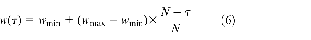
where N is the maximum number of iterations, and $ω_{min}$ and $ω_{\max}$ are the minimum and maximum inertial factors, respectively. Typically, $ω_{min}$ = 0.4 and $ω_{\max}$ = 0.9.²⁰ The APSO with the linearly decreasing inertial weight is called ωAPSO. The flow chart of ωAPSO is shown in Figure 2.

Figure 2.

The flow chart of ωAPSO.

ABC algorithm principles

ABC is based on the foraging behavior of honeybees. In the ABC algorithm, three specific roles are allocated to artificial bees, namely, the scout bee, the employed forager, and the onlooker bee. Importantly, each artificial bee is restricted to a single role at any given time; however, role transitions are permissible based on the bee’s status during the solution process. Scout bees assume the duty of conducting a global random search within the solution space of ABC. Furthermore, employed foragers serve a dual purpose: they not only direct the swarm towards the global optimal solution but also search for superior nectar sources proximate to their existing discoveries. Moreover, these employed foragers provide pivotal information to onlooker bees. Relying on this information, onlooker bees engage in localized searches around the identified nectar sources, with higher nectar concentrations increasing their likelihood of being targeted. In the vicinity of a honey source, when onlooker bees discover an alternative source that surpasses the existing one in quality, a role reversal occurs between the onlooker bee and the employed forager.

The ABC algorithm commences with an initial search phase executed by scout bees. During this phase, these bees strive to explore the entire problem solution space as comprehensively as possible to ensure a rich diversity of solutions. Subsequently, the nectar concentrations of various sources are assessed and recorded. Consequently, the algorithm transitions to the employed forager search phase. Given that the initial nectar sources represent the best finds of each scout bee, this information becomes invaluable in guiding the swarm’s search direction. Thus, all scout bees morph into employed foragers. During this phase, each employed forager conducts a targeted search in the vicinity of its previously discovered nectar source. Following this, a comparison is made between the newly identified and the existing nectar sources, and the one with a higher concentration is selected.

Lastly, the algorithm enters the onlooker bee search stage. Onlooker bees choose their search locations based on the nectar concentration data supplied by employed foragers. Evidently, sources with higher concentrations have a greater probability of selection. During this stage, each onlooker bee performs a localized random search around its selected nectar source. Subsequently, the algorithm compares the newly discovered source with the existing one. The source demonstrating superior concentration becomes the new nectar source, while less optimal sources are eliminated. If an onlooker bee identifies a local optimum, it assumes the role of an employed forager, thereby initiating a role-switch with the former employed forager – now re-designated as an onlooker bee.²¹

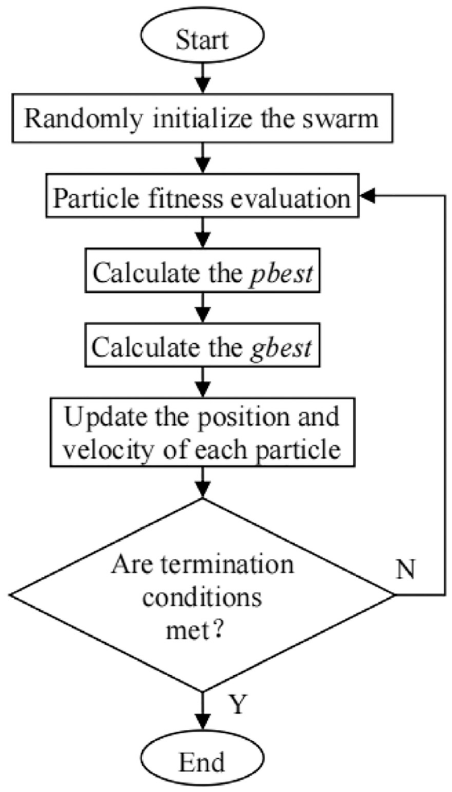
In summary, the distinguishing feature of the ABC algorithm lies in its balanced approach to guided random searches. This strategy harmonizes the utility of historical data with the element of randomness. Additionally, it carefully considers both the convergence rate and the population diversity within the algorithm’s framework. ABC retains high-quality feasible solutions and eliminates poor feasible solutions in continuous iterative. The flow chart of ABC is shown in Figure 3.

Figure 3.

The flow chart of ABC.

ABC-ωAPSO algorithm and stability analysis

The improved PSO greatly depends on the global optimal solution in the late iteration; this dependence weakens the randomness of the algorithm. Therefore, the onlooker bee search factor in the bee colony was introduced to strengthen the ωAPSO.

The onlooker bee search is based on using a roulette to randomly select individuals and then conduct greedy search around them. In the ABC algorithm, the onlooker bee also undergoes a meticulous decision-making process. After searching the space surrounding a discovered nectar source, the onlooker bee compares its findings with the existing source. If the newly identified nectar source boasts a higher concentration, the bee transitions to this new source, abandoning the old one. Conversely, if the old source proves to be more abundant, the bee remains. Through ongoing comparisons, the onlooker bee consistently retains the better options. This search pattern is both random and pioneering.²² In the hybrid algorithm, the pbest is considered as the employed forager in ABC, and onlooker bees conduct greedy search around it. The ωAPSO introduced with onlooker bees in ABC is denoted as ABC-ωAPSO. The introduction of onlooker bees does not reduce the stability of the algorithm because they constantly select better individuals for the next generation of population during the search; hence, the whole population develops in the optimal direction. The flow chart of ABC-ωAPSO is shown in Figure 4.

Figure 4.

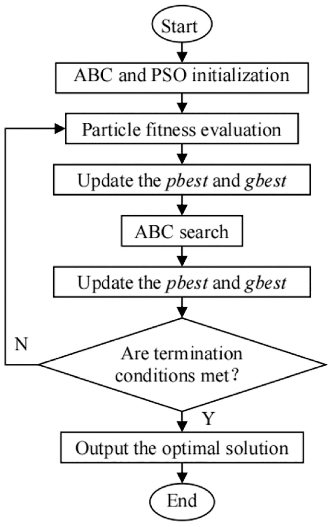
The flow chart of ABC-ωAPSO.

The initial terrain matching in ABC-ωAPSO proceeds as follows:

1. Set the global initialization domain U.

U = {(x, y) | | x - x_{1}^{p} | < 3 σ_{x}, | y - y_{1}^{p} | < 3 σ_{y}}

(7)

where [ $x_{1}^{p}, y_{1}^{p}$ ] is the first point of INS track, $σ_{x}$ and $σ_{y}$ are standard deviations of prior position error.

2. Random initialization of ABC and PSO swarm. Set the maximum number of iterations, number of swarms, and particles as $ω$ , c₁, and c₂.

3. Calculate the fitness-function value of each particle.

4. Update the pbest and gbest.

5. ABC search. Onlooker bees implement a greedy search around pbest. Onlooker bees judge whether the current position is the optimal position corresponding to the minimum fitness-function value.

6. Update the pbest and gbest.

7. Judge whether the termination conditions are met. If termination conditions are met, record the optimal matching sequence. Otherwise, loop to step 3 until termination conditions are met. The termination condition is that the maximum number of iterations or the matching result satisfies the limit difference.

ABC-ωAPSO is applied to terrain initial matching. The initial matching results are refined using the improved ICCP. The algorithm after two matchings is denoted as ICCP-a.

Simulation and analysis

Parameter setting

To verify the performance of traditional ICCP-a, three tests were conducted in this paper. For comparative analysis, the ICCP-a algorithm was benchmarked against traditional ICCP and TERCOM-ICCP algorithms. TERCOM-ICCP combines the capabilities of TERCOM for initial rough matching and ICCP for the subsequent fine matching phase.

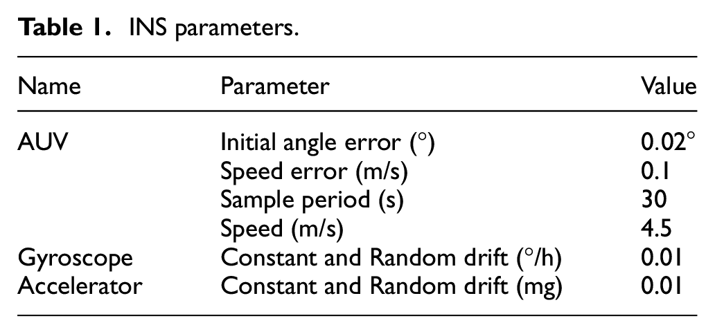
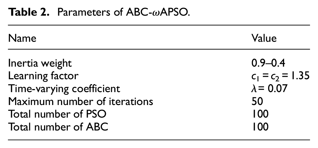
Three tests were conducted to evaluate the performance of these algorithms, each with distinct initial conditions. For Test 1 and Test 2, the initial geographical coordinates were 122.086°E, 37.577°N, the initial course was 150° north by east, and the initial errors of the INS were 0.35′ and 0.55′ to the east, 0.35′ and 0.55′ to the north, respectively. Test 3, however, focused on assessing the algorithms under varying terrains. The AUV traveled at a uniform speed through two distinct regions. The initial errors in the INS were 0.2′ to the east, 0.2′ to the north, and the initial course was 10° north by east. The region with more pronounced terrain changes was labeled as “area-a,” where the standard deviation in water depth was 1.41. Conversely, “area-b,” exhibiting less dramatic terrain changes, had a water depth standard deviation of 0.62. The initial positions for these regions were 122.07°E, 37.575°N and 122.07°E, 37.585°N, respectively. The INS parameters are tabulated in Table 1. The parameter settings of ABC-ωAPSO are provided in Table 2.

Table 1.

INS parameters.

Name	Parameter	Value
AUV	Initial angle error (°)	$0.02 °$
	Speed error (m/s)	0.1
	Sample period (s)	30
	Speed (m/s)	4.5
Gyroscope	Constant and Random drift (°/h)	0.01
Accelerator	Constant and Random drift (mg)	0.01

Table 2.

Parameters of ABC-ωAPSO.

Name	Value
Inertia weight	0.9–0.4
Learning factor	c ₁ = c₂ = 1.35
Time-varying coefficient	$λ$ = 0.07
Maximum number of iterations	50
Total number of PSO	100
Total number of ABC	100

Test trajectory and analysis

Test 1: The underwater vehicle turned at a uniform speed. Figures 5 and 6 provide graphical representations of the trajectories produced by these three matching algorithms, offering visual insights into their comparative performance.

Figure 5.

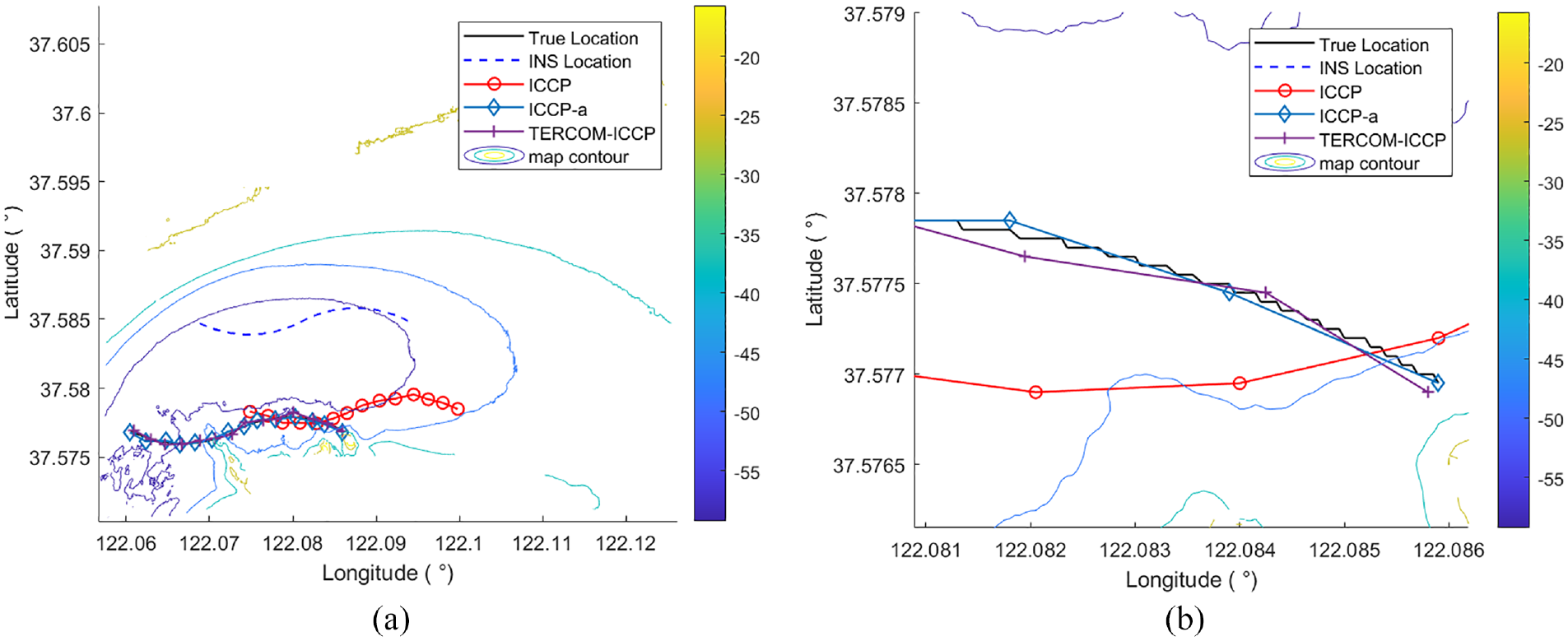
Matching results with an initial position error of (0.35′, 0.35′): (a) Initial INS error of (0.35′, 0.35′) and (b) locally enlarged image with an initial error of (0.35′, 0.35′).

Figure 6.

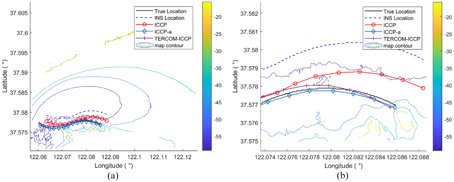
Matching results with an initial position error of (0.55′, 0.55′): (a) Initial INS error of (0.55′, 0.55′) and (b) locally enlarged image with an initial error of (0.55′, 0.55′).

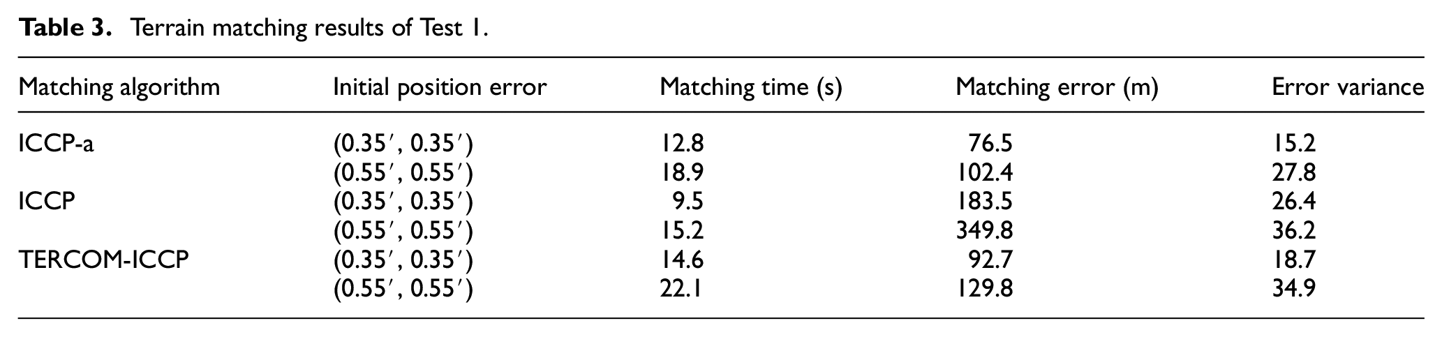
Figures 5 and 6 delineate a comparison among ICCP-a, TERCOM-ICCP, and traditional ICCP algorithms. In both instances of varying initial errors, ICCP-a and TERCOM-ICCP markedly outperform the traditional ICCP. Further scrutiny, particularly through local magnification, reveals that ICCP-a offers greater stability in matching than TERCOM-ICCP. The matching times, matching errors, and matching error variances of the three algorithms are compared in Table 3. The matching error is expressed as the mean value of the root mean square of the error in the longitude and latitude directions of the entire track sequence.

Test 2: The underwater vehicle traveled straight at a uniform speed. Figure 7 shows the trajectory of three matching algorithms.

Table 3.

Terrain matching results of Test 1.

Matching algorithm	Initial position error	Matching time (s)	Matching error (m)	Error variance
ICCP-a	(0.35′, 0.35′)	12.8	76.5	15.2
ICCP-a	(0.55′, 0.55′)	18.9	102.4	27.8
ICCP	(0.35′, 0.35′)	9.5	183.5	26.4
ICCP	(0.55′, 0.55′)	15.2	349.8	36.2
TERCOM-ICCP	(0.35′, 0.35′)	14.6	92.7	18.7
TERCOM-ICCP	(0.55′, 0.55′)	22.1	129.8	34.9

Figure 7:

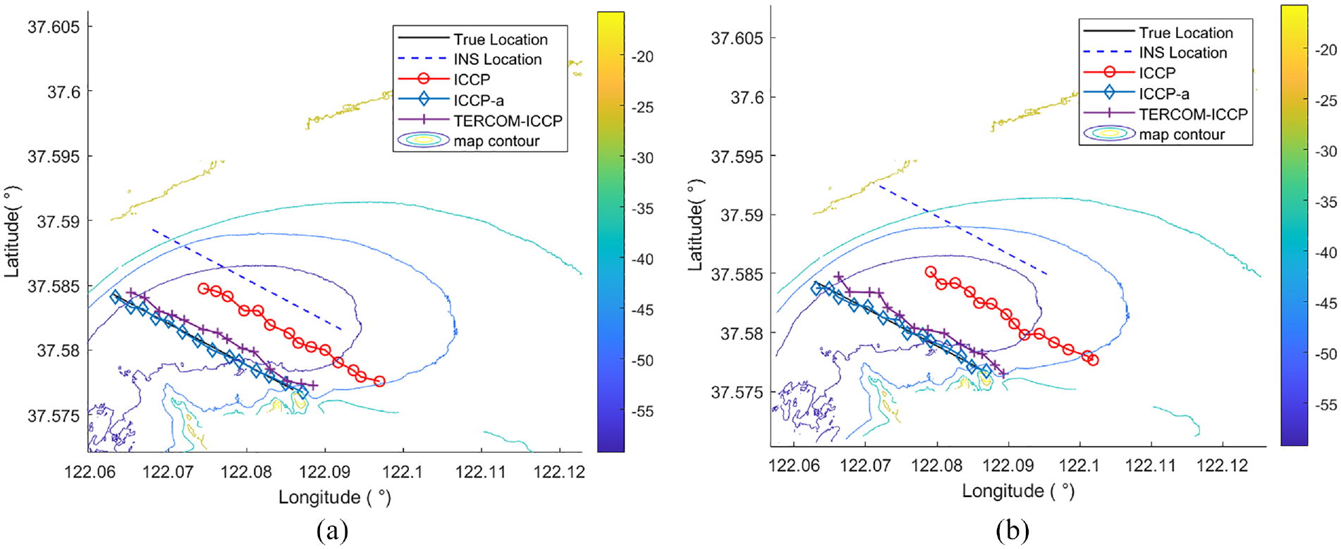
Matching results of three matching algorithms of Test 2: (a) Initial INS error of (0.35′, 0.35′) and (b) initial INS error of (0.55′, 0.55′).

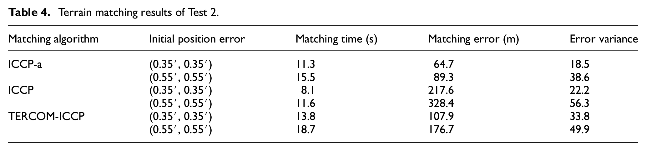
As depicted in Figure 7, when considering two distinct scenarios of initial error, the performance of ICCP-a in terms of matching is markedly superior to both ICCP and TERCOM-ICCP. Furthermore, as the initial error escalates, it becomes evident that the conventional models of ICCP and TERCOM-ICCP exhibit diminished stability. In contrast, ICCP-a maintains a commendable level of stability under the same conditions. Table 4 compares the matching times, matching errors, and matching error variances of the three algorithms.

Test 3: The underwater vehicle traveled straight at a uniform speed. Figures 8 and 9 present the trajectory analysis for three distinct matching algorithms within terrain areas labeled as area-a and area-b.

Table 4.

Terrain matching results of Test 2.

Matching algorithm	Initial position error	Matching time (s)	Matching error (m)	Error variance
ICCP-a	(0.35′, 0.35′)	11.3	64.7	18.5
ICCP-a	(0.55′, 0.55′)	15.5	89.3	38.6
ICCP	(0.35′, 0.35′)	8.1	217.6	22.2
ICCP	(0.55′, 0.55′)	11.6	328.4	56.3
TERCOM-ICCP	(0.35′, 0.35′)	13.8	107.9	33.8
TERCOM-ICCP	(0.55′, 0.55′)	18.7	176.7	49.9

Figure 8.

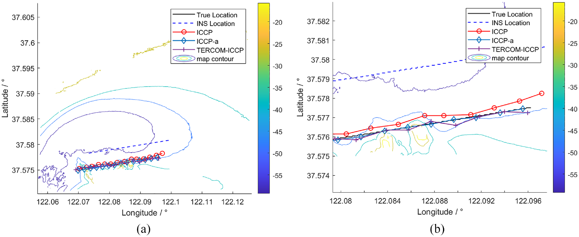
Matching results with an initial position error of (0.2′, 0.2′) in area-a: (a) Initial INS error of (0.2′, 0.2′) in area-a and (b) locally enlarged image with an initial error of (0.2′, 0.2′) in area-a.

Figure 9.

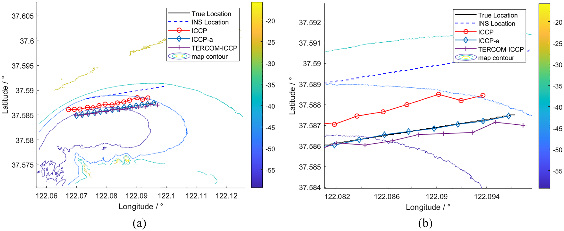
Matching results with an initial position error of (0.2′, 0.2′) in area-b: (a) Initial INS error of (0.2′, 0.2′) in area-b and (b) locally enlarged image with an initial error of (0.2′, 0.2′) in area-b.

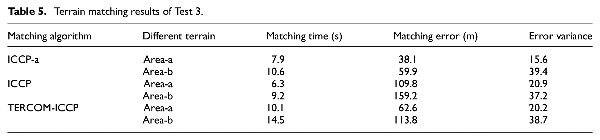
As shown in Figure 8, all three algorithms – ICCP-a, traditional ICCP, and TERCOM-ICCP – exhibit commendable performance in areas with substantial terrain variations. Nonetheless, a more granular inspection via local magnification clearly reveals that ICCP-a stands out for its stability and unmatched accuracy. In stark contrast, the traditional ICCP lags significantly in areas with less pronounced terrain changes. The instability of TERCOM-ICCP is even more conspicuous in these areas. However, ICCP-a excels in its consistency and superior matching capability across different terrain types. Table 5 compares the matching times, matching errors, and matching error variances of the three algorithms.

Table 5.

Terrain matching results of Test 3.

Matching algorithm	Different terrain	Matching time (s)	Matching error (m)	Error variance
ICCP-a	Area-a	7.9	38.1	15.6
ICCP-a	Area-b	10.6	59.9	39.4
ICCP	Area-a	6.3	109.8	20.9
ICCP	Area-b	9.2	159.2	37.2
TERCOM-ICCP	Area-a	10.1	62.6	20.2
TERCOM-ICCP	Area-b	14.5	113.8	38.7

To further evaluate the performance of the algorithm, the matching effect of ICCP-a under different measurement noises were tested. All algorithms were subjected to the addition of different white noises to the initial position error of Test 2, which was (0.35′, 0.35′). The added white noises approximately followed a normal distribution, namely, N(0,1), N(0,4), and N(0,9), respectively. The matching errors are presented in Table 6.

Table 6.

Matching errors under different noises.

Matching algorithm	Matching error (m)
Matching algorithm	N(0,1)	N(0,4)	N(0,9)
ICCP-a	64.7	68.3	75.1
ICCP	217.6	243.2	279.5
TERCOM-ICCP	107.9	130.4	163.7

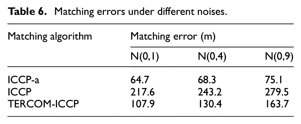
From Table 6, it can be observed that as the noise level increases, the matching errors of all three algorithms also increase. However, ICCP-a exhibits the slowest rate of change, clearly indicating that increasing the Mahalanobis distance effectively reduces the impact of noise on ICCP. Moreover, compared with the other two algorithms, ICCP-a demonstrates the highest matching accuracy under the three different noise conditions.

We also conducted a study on the iterative process of the algorithm with an initial position error of (0.35′, 0.35′) in Test 2. ICCP-a had 50 iterations for coarse matching and 10 iterations for fine matching. For a fair comparison, ICCP was set to have 60 iterations, and in the TERCOM-ICCP, ICCP had 10 iterations. All three algorithms ceased searching once the maximum number of iterations was reached. Figure 10 illustrates the matching errors at each iteration of the three algorithms.

Figure 10.

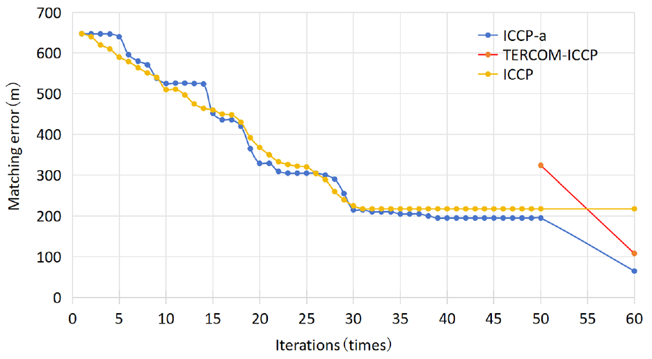
Matching errors of three algorithms in the iterative process.

In the ICCP-a, when using ABC-ωAPSO for initial matching, there are two noticeable decreases in matching errors, representing improvements in both PSO and ABC searches. This strongly demonstrates that PSO based on ABC search can effectively enhance global optimization capabilities. When the number of ICCP iterations reaches 30 times, there is no significant change in matching errors. In the TERCOM-ICCP, the initial matching error with the TERCOM is 324.6 m, and ICCP iterations are performed based on the matching result of TERCOM. Figure 10 illustrates that using both algorithms results in lower matching errors compared to using just one algorithm. The matching accuracy is higher when ABC-ωAPSO is used for initial matching than when TERCOM is employed.

In conclusion, our multi-faceted experiments establish the superior performance of ICCP-a and TERCOM-ICCP over the traditional ICCP. This assertion gains quantitative backing from Tables 3 and 4, which indicate that with initial INS errors of (0.35′, 0.35′), the matching error with ICCP-a was reduced by up to 3.4 times compared to the traditional ICCP, and by 1.7 times compared to TERCOM-ICCP. As these initial errors escalated to (0.55′, 0.55′), ICCP-a further reinforced its superior standing by reducing matching errors by as much as 3.7 and 2 times, respectively. The predominance of ICCP-a can be attributed largely to its resilience to course errors – a shortcoming that severely affects TERCOM-ICCP. In scenarios where the course error is excessively large, TERCOM exhibits a phenomenon of mismatching. Consequently, the rough matching effect of ABC-ωAPSO outshines that of TERCOM.

Test 3 reveals that all three algorithms exhibit enhanced performance in regions characterized by pronounced terrain variations. However, in areas where the terrain changes are subtle, the matching error for the traditional ICCP noticeably escalates, and instability becomes evident in TERCOM-ICCP. This occurs primarily because these less variegated terrains have an abundance of similar topographical areas, making mismatches more likely.

In contrast, ICCP-a demonstrates robust matching capabilities across both types of terrains, thus underscoring the benefits of its double-matching feature. Additionally, by utilizing ABC-ωAPSO for the initial matching phase, the algorithm effectively minimizes initial position errors, setting the stage for more precise fine matching via the ICCP algorithm. When considering the time required for matching, ICCP-a does not show a significant increase, thereby affirming the rapid global optimization capabilities of ABC-ωAPSO. Furthermore, even when the noise level is increased, ICCP-a also exhibits remarkable stability. Importantly, ICCP-a achieves superior positional accuracy, meeting the stringent navigational requirements of AUVs for extended voyages. This makes it highly valuable for realizing the goal of autonomous passive navigation in AUVs.

Conclusions

To resolve the sensitivity of the traditional ICCP to the initial position error, this study proposes an improved terrain-aided matching algorithm that combines coarse and fine matching. The two-step matching reduces the initial position error before fine matching. First, the Mahalanobis distance replaces the Euclidean distance in ICCP to relax the assumption of noiseless depth data in ICCP, thereby improving the practical value of the algorithm. Second, because ICCP has good refinement ability but poor global-search ability, the ABC-ωAPSO is introduced for rough matching, and the improved ICCP is then applied for fine matching. In the improved algorithm, termed ICCP-a, the second matching effect improves the positioning accuracy of the single matching algorithm. Finally, ωAPSO and ABC are combined effectively to improve the global optimization ability of the traditional PSO. ABC-ωAPSO can better help the traditional ICCP to reduce the initial INS position error, thus realizing the perfect combination of ABC-ωAPSO with ICCP.

Footnotes

Declaration of conflicting interests

The author(s) declared no potential conflicts of interest with respect to the research, authorship, and/or publication of this article.

Funding

The author(s) disclosed receipt of the following financial support for the research, authorship, and/or publication of this article: The work is supported by The National Natural Science Foundation of China [grant number 51979047], The Natural Science Foundation of Heilongjiang Province of China [grant number YQ2021E011].

ORCID iD

Dan Wang

References

Zhao

Zhou

. Cooperative target location method based on master-slave autonomous underwater vehicles mobile network. Electron Inf Technol 2022; 44(6): 1919–1926.

Fang

Huang

, et al. AUV position tracking and trajectory control based on fast-deployed deep reinforcement learning method. Ocean eng 2022; 245: 110452.

Guo

, et al. Underwater navigation methodology based on intelligent velocity model for standard AUV. Ocean eng 2020; 202: 107073.

Guo

Liu

Fan

, et al. Research progress of path planning methods for autonomous underwater vehicle. Math Probl Eng 2021; 2021: 1–25.

Sheng

Zhang

, et al. Underwater terrain-aided navigation system based on combination matching algorithm. ISA Trans 2018; 78: 80–87.

Han

Wang

Deng

, et al. A combined matching algorithm for underwater gravity-aided navigation. IEEE-ASME Trans Mechatron 2018; 23(1): 233–241.

Ren

Wang

Lin

, et al. Improved iterative closest contour point matching navigation algorithm based on geomagnetic vector. Electronics 2022; 11(5): 796.

Liu

Lin

, et al. Gravity aided positioning based on real-time ICCP with optimized matching sequence length. IEEE Access 2019; 7: 97440–97456.

Wang

Deng

Zhang

, et al. An improved ICCP gravity matching algorithm based on Mahalanobis distance. In: 40th Chinese Control Conference (CCC), Shanghai, China, 2021, pp. 3503–3508. New York: IEEE.

10.

Wang

Zhang

. Multipath parallel ICCP underwater terrain matching algorithm based on multibeam bathymetric data. IEEE Access 2018; 6: 48708–48715.

11.

Chen

Song

. Improved particle swarm optimization geomagnetic matching algorithm based on simulated annealing. IEEE Access 2020; 8: 226064–226073.

12.

Gao

Zhao

Zhou

, et al. Improved artificial bee colony algorithm based gravity matching navigation method. Sensors 2014; 14(7):12968–12989.

13.

Wang

, et al. An innovative PSO-ICCP matching algorithm for geomagnetic navigation. Measurement 2022; 193: 110958.

14.

Yuan

Zhang

Yuan

, et al. A combinational underwater aided navigation algorithm based on TERCOM/ICCP and Kalman Filter. In: 4th International Joint Conference on Computational Sciences and Optimization (IJCCSO), Kunming and Lijiang City, China, 2011, pp. 952–955. New York: IEEE.

15.

Ding

Cheng

. A new contour-based combined matching algorithm for underwater terrain-aided strapdown inertial navigation system. Measurement 2022; 202: 111870.

16.

Zhang

, et al. An improved ICCP-based underwater terrain matching algorithm for large initial position error. IEEE Sens J 2022; 22(16): 16381–16391.

17.

Wang

Zhu

Qin

, et al. Matching error of the iterative closest contour point algorithm for terrain-aided navigation. Aerosp Sci Technol 2018; 73: 210–222.

18.

Jiang

Wei

Shao

, et al. Research on large-scale bi-level particle swarm optimization algorithm. IEEE Access 2021; 9: 56364–56375.

19.

Song

Cao

. An improved particle swarm optimization algorithm with adaptive weighted delay velocity. Syst Sci Control Eng 2021; 9(1): 188–197.

20.

Shi

Eberhart

. Empirical study of particle swarm optimization. In: Proceedings of the 1999 Congress on Evolutionary Computation-CEC99 (Cat. No. 99TH8406), Washington, DC, 1999, pp. 1945–1950. New York: IEEE.

21.

Sharma

Kumar

Sharma

. Improved Gbest artificial bee colony algorithm for the constraints optimization problems. Evol Intell 2021; 14(3): 1271–1277.

22.

Chu

Cai

Gao

, et al. An artificial bee colony algorithm with adaptive heterogeneous competition for global optimization problems. Appl Soft Comput 2020; 93: 106391.

Underwater terrain-matching algorithm based on improved iterative closest contour point algorithm

Abstract

Keywords

Introduction

ICCP and improvement

ICCP algorithm

Improved ICCP algorithm

ABC-ωAPSO terrain-matching algorithm

Improved PSO algorithm

ABC algorithm principles

ABC-ωAPSO algorithm and stability analysis

Simulation and analysis

Parameter setting

Test trajectory and analysis

Conclusions

Footnotes

Declaration of conflicting interests

Funding

ORCID iD

References