Sage Journals: Discover world-class research

Abstract

Vision recognition and RFID perception are used to develop a smart AGV travelling on fixed paths while retaining low-cost, simplicity and reliability. Visible landmarks can describe features of shapes and geometric dimensions of lines and intersections, and RFID tags can directly record global locations on pathways and the local topological relations of crossroads. A topological map is convenient for building and editing without the need for accurate poses when establishing a priori knowledge of a workplace. To obtain the flexibility of bidirectional movement along guide-paths, a camera placed in the centre of the AGV looks downward vertically at landmarks on the floor. A small visual field presents many difficulties for vision guidance, especially for real-time, correct and reliable recognition of multi-branch crossroads. First, the region projection and contour scanning methods are both used to extract the features of shapes. Then LDA is used to reduce the number of the features' dimensions. Third, a hierarchical SVM classifier is proposed to classify their multi-branch patterns once the features of the shapes are complete. Our experiments in landmark recognition and navigation show that low-cost vision systems are insusceptible to visual noises, image breakages and floor changes, and a vision-based AGV can locate itself precisely on its paths, recognize different crossroads intelligently by verifying the conformance of vision and RFID information, and select its next pathway efficiently in a bidirectional flow network.

Keywords

Automated Guided Vehicle Vision Guidance Landmark Recognition Navigation Control

1. Introduction

Flow-path network design is the first step in developing an automated guided vehicle (AGV) system at the strategic level [1]. The flow-path layout consists of the fixed guide-paths on which vehicles can travel to the various points for picking up and delivering loads. Its flow topology describes the complexity of the guide-path network, e.g., a simple case of one single loop versus a complicated network with paths, crosses, shortcuts and junctions, influenced by different application requirements, such as the number of AGVs used, the number of transportation requests, the degree of the occupancy of the AGVs, the distances to be travelled and the number of pick-up and delivery points [2].

A guide-path layout is often represented by a directed network in which aisle intersections and pick-up and delivery locations can be considered as nodes. Its design focuses on the flow topology, not including the navigation infrastructure, which uses different landmarks to describe lines and nodes of the flow network. Typically, lines (paths) are specified by electric wires buried in the floor. Wires carry AC electric signals, which can be detected by the AGV's on-board antenna. Multiple pathways and crossroads are recognized by using different alternation frequencies. Vehicles are restricted to their specified path in order to avoid losing guiding signals, termed fixed-path guidance. Rather than using fixed paths, the other AGVs can deviate significantly from their guide-paths and their preferred tracks are software programmed, which is known as free-ranging. They navigate based on their own location, e.g., using the triangular computation of returning lasers reflected from more than three fixed reflectors on a wall [3, 4] or by using the correlation computation of the texture features of concrete floors with respect to a large-scale visual record [5], and path planning on grid maps or feature maps. For AGV navigation, depending on artificial landmarks, they need to be put in different locations, and a map of their positions has to be built and uploaded into the central computer. If the facility's layout is frequently changed, the repeated process of map building is rather tedious and prone to errors. Simultaneous localization and mapping (SLAM) [6, 7] is widely used in robotics, where a vehicle is located in an unknown environment and it is capable of building a map of the environment while estimating its position and orientation within this map at the same time. Monocular SLAM and visual servo are combined in [8] to form a hybrid control approach that contains a position-based control for global navigation and an image-based visual servo for fine motions needed for an AGV to accurately steer towards a loading/unloading point. It can bypass the need for artificial landmarks or an accurate map of the environment.

Although a free-ranging AGV is often considered to be more adaptable and intelligent due to its motion freedom, its advantages may be not so apparent in many industries, e.g., its freedom is constrained by finite-space environments, or if its reflective laser is obstructed by other equipment, or if vehicles interfere with each other when there are a lot of them lacking ordered guidance through aisles. Besides, equipment expense is also an obstacle to extensively using AGVs in cost-sensitive industries. In practice, fixed guide-paths are still widely used in many large-scale AGV systems. Vehicles can travel in only one direction (unidirectional) or both directions (bidirectional). Advances in technology and cost reduction in microelectronics and microcomputers allow for the development of smart AGVs for fixed paths, which can store routing instructions, make decisions and even take part in controlling the traffic of the global system. Should smart fixed-path AGVs or free-ranging AGVs be selected to establish a large-scale AGV system? It would be best to make a trade-off between flexibility and efficiency, system scale and vehicle expense, individual intelligence and conflict.

Visually recognizing artificial landmarks can help the AGV acquire rich guide information, which is useful for increasing its intelligence. Vision guidance using an on-board camera is a promising technology [9 –13] that can attain high flexibility or easy reconfiguration while retaining low-cost, simplicity and reliability in industrial systems. Line tracking is a low-cost vision-based approach for detecting and following guide-paths, where the computational load resulting from visual recognition is avoided by learning or coding the specific perceptual knowledge that the AGV is expected to extract from the environment via artificial landmarks [9, 10]. Guidance may also be related to the visual servo of mobile robots for pallet engagement, where position information is fused from the laser and the camera [12], or from just the camera [13].

Asides from unidirectional or bidirectional paths, crossroads are common elements in complex guide-path networks. Turning around on multi-branch crossroads requires not only movement control but also intelligent recognition (for intersections) and decisions (path selection). Although this can be done by using electric wires of different alternation frequencies or intersected magnetic tapes, this is only effective when carrying out arc-path turning. The turning radius of an AGV is determined by the physical size of the vehicle, potentially leading to additional space requirements. Vision perception has already been used for crossroads. In order to broaden the AGV's visual field and detect landmarks in front of it as early as possible, the camera is placed on the AGV facing obliquely downwards and ahead [14 –16]. The width and number of paths are detected by sampling a single row of pixels at the top of the image, which is used to judge whether a crossroads exists [14]. It is simple and easy to implement but sensitive to the AGV's pose at the intersections. The AGV in [15] preserves a mass of scene templates and matches the real-time images acquired in the turning process with these templates. Hough transformation is simultaneously used in [16] to detect lines and circles so as to distinguish the forward path and turning path. Both of them [14, 15] need a large volume of memory and intensive computing capacity. Other common problems include the restriction of unidirectional movement and the lack of consideration of image interference.

In practice, vision guidance has not been used as broadly as wired or magnetic guidance in industry. In order to convince industrial practitioners of the virtues of computer vision, intelligent recognition and decision mechanisms for a low-cost vision guidance system are developed for an AGV operating in complex flow networks where a mix of unidirectional and bidirectional paths are used for simple traffic control and high transportation efficiency, and the AGV uses quarter turning to adapt to a finite space. The AGV can intelligently recognize different crossroads, select its next path and track its guide-paths until it arrives at its destination. System configuration and infrastructure building are introduced in section 2. A framework for the intelligent navigation of AGVs on fixed paths is proposed in section 3. The paper focuses on crossroads recognition which uses computer vision and path selection based on visible features of the intersections and topological information of the crossroads. Section 4 discusses computer vision techniques for classifying intersections, including feature extraction, dimensionality reduction and pattern recognition. In section 5, we construct an example of a bidirectional flow network, and carry out an intelligent navigation experiment. A brief conclusion in section 6 summarizes our current work as well as potential improvements.

2. System configuration

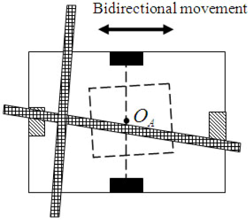
As shown in Figure 1, two driving wheels are placed symmetrically on both sides of the AGV, and the geometric centre, O_A, is the middle point of the wheel axis. An on-board camera is mounted on the centre of the AGV, O_A, vertically, looking downwards at the landmarks on the floor. This method of installing the camera means it can track guide-paths in both directions, but also that it has a relatively small visual field. If the AGV cannot detect and recognize an intersection promptly at a crossroads, the landmark will move out of its visual field and the AGV may miss the correct pathway.

Figure 1.

AGV structure

Visible tapes and RFID tags are used as landmarks to construct the infrastructure for visual navigation. Each visible tape stuck to the floor represents a guide-path, which is used by the vision system as a reference line to measure AGV deviations with respect to its guide-path at its position and orientation. An intersection of several pieces of tape means that it is a crossroads of multiple pathways, which is used not only as a multi-branch pattern to describe the pathway topology of crossroads, but also as a reference point to measure the AGV's pose deviations at pick-up and delivery sites. Due to its small visual field, the on-board camera only looks at the local features of guide-paths. It is difficult for the vision system to find the absolute location of the AGV in a flow network. One possible solution is to pre-set the initial location of the flow network for the AGV, and then to infer its next location by dead reckoning its incremental motion according to geometric maps. However, the accumulated data of dead reckoning tends to drift due to wheel slippage. It is often necessary to reset the counters of dead reckoning by using some artificial landmarks. Besides, building and updating geometric maps need lots of accurate, detailed geometric information, e.g., path length and point location, so mapping is rather time-consuming and inconvenient.

Another possible solution is to use RFID tags to describe absolute locations and other abstract information directly. Although the vision system is adept at detecting visible geometric information (pose deviations and multi-branch patterns), its efficiency at recognizing abstract information (a string of characters) is not as high as that of a RFID reader. A series of RFID tags are used to indicate path number, crossroads number (with pathway topology), milestone number and station number, as well as some control functions attached to specific pathways, which are called pathway tags, intersection tags, milestone tags, station tags and control tags. Visible landmarks (tapes and intersections) on the floor can easily correspond to abstract symbols (nodes, paths and crossroads) on a topological map. Instead of storing accurate geometric information, the topological map only describes the connection between nodes and paths. It is relatively convenient to build and maintain a topological map compared to a geometric map.

An example of a topological map for a bidirectional flow network is shown in Figure 2. Each path segment of two nodes (e.g., stations and/or intersections) is defined as a separate pathway, numbered a, b… in Figure 2 and stored using pathway tags. Milestone tags are used to record the specific absolute positions of a pathway. With the help of two tags, the AGV can discriminate one guide-path from another and locate itself conveniently on different parts of a pathway by using dead reckoning. The intersection tag describes the local topology relation at a crossroads of how some pathways converge to a point, e.g., the adjacency and connectivity of the pathways, and the angle between two pathways. In Figure 2 it can be seen that pathway a is adjacent to pathways b and d, and their angles are α₁ and α₄. The station tag is used to denote an operating position, and usually some operations with other facilities are assigned, e.g., picking up and laying down loads. Control tag records control functions to change the travelling states of AGV on its guide-path, e.g., accelerating or slowing down.

Figure 2.

A topological map of a bidirectional flow network

In Figure 2, the crossroads are an important element in the AGV's navigation on fixed paths, which defines the relation between different pathways. Both an intersection of several tapes and a RFID tag are used to describe visible information (pose deviations and multi-branch patterns) and abstract information (pathway topology) respectively. This method of arranging vision and RFID sensors is done in order to improve the accuracy, reliability and real-time performance of low-cost guidance systems. Many attempts have been made to improve the accuracy of robot location by using the RFID technique or combining it with other techniques, e.g., utilizing the read time for the antenna to detect a tag in a gird-like pattern of many passive RFID tags (the average location error is about 6 cm for a grid-like pattern of 4.2m×6.2m with a spacing of 34 cm) [17], or by fusing the location data of the odometry and wireless sensor network to deal with the unbounded accumulated error of dead reckoning (the average square deviation is about 0.81 m² for an area of 30m×30m) [18]. Its accuracy and repeatability (in a large area) are not sufficient for industrial applications. However, an on-board camera can measure the position of an intersection in its visual field to the accuracy of a millimetre. Since the AGV is required to dock accurately on the intersections of crossroads (needed for turnaround control, discussed in section 3), it is necessary to use the vision system to locate the AGV at precise positions. In order to enhance the real-time performance of guidance systems, a priori knowledge (e.g., an angle of two pathways) is stored in RFID tags directly, although the vision system can measure this angle based on vector graphs. Asides from this, the multi-branch pattern recognized by the vision system should agree with the pathway topology recorded by RFID tags. This mutual verification mode is beneficial to the reliability of guidance systems on complex guide-paths.

Electric wires and magnetic tapes have already been used to form intersections of several arc pathways, as shown in Figure 3. It is convenient to recognize different pathways by measuring the alternation frequencies of electric wires or by finding disperse points of magnetic signals. However, the approach is only suitable for arc-shaped crossroads, not for square-shaped crossroads, as shown in Figure 4. The latter is especially useful in finite-space environments. For example, it is difficult for an AGV with a body size of 1.9m×0.9m to go through a door with a width of 1.4m and to enter a corridor with a width of 2m on arc paths, so quarter turning on square-shaped crossroads has to be used [19]. After the AGV locates its centre, O_A, in the intersection, it can turn around this point with a radius of zero, which is called self-revolving around its centre. It needs a much smaller space than turning on an arc-shaped crossroads. Another obvious merit of square-shaped crossroads is that they can easily contain more pathways from different directions, so it is especially suitable for constructing multi-branch crossroads of a complex flow-path network.

Figure 3.

Arc-shaped crossroads

Figure 4.

Square-shaped crossroads

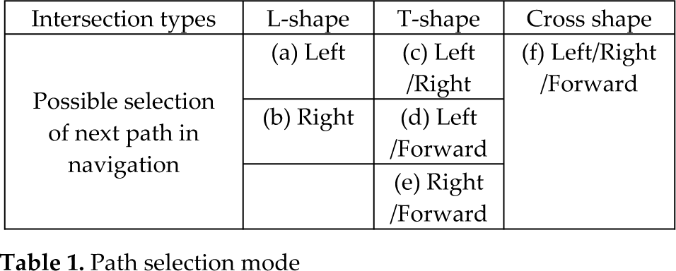
As shown in Figure 4, L-shapes, T-shapes and cross shapes are three common types of square-shaped crossroads. When an AGV arrives at intersections of guide-paths with different directions, the mode of path selection is determined by the crossroads' topology and the motion direction together, as shown in Table 1. For the L-shaped intersections shown in Figure 4.(a) and (b), there is only one next possible path that can be selected, the left pathway or the right pathway. For the T-shaped intersections shown in Figure 4.(c), (d) and (e), there are two potential next paths. If the intersection is a cross shape, three directions are all possible: left, right and forward. At this time, the AGV selects an optimal path as its next track when there is more than one optional branch, according to its location and destination.

Table 1.

Path selection mode

Intersection types	L-shape	T-shape	Cross shape
Possible selection of next path in navigation	(a) Left	(c) Left/Right	(f) Left/Right/Forward
	(b) Right	(d) Left/Forward
		(e) Right/Forward

3. Intelligent navigation framework

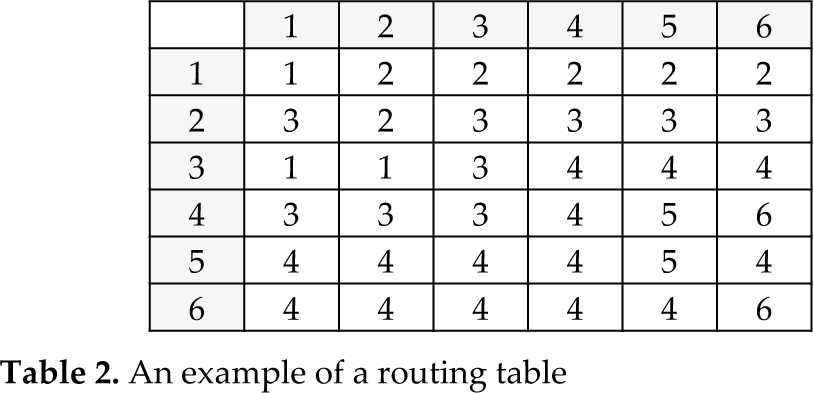
As mentioned above, visible tapes and RFID tags are used to build the navigation infrastructure, and a topological map is developed to describe the flow-path network. In order to take both individual intelligence and equipment complexity into account, the intelligent navigation of a whole AGV system is divided into different stages and levels, as shown in Figure 5. At a system level, there are three stages of design, planning and operation. AGV system design includes guidance technology selection and infrastructure setup, guide-path design and map building. In order to facilitate the creation and editing of a topological map in an interactive manner, the visualized map-building software is developed on the central computer. The user can build a map quickly by drawing lines and points, and inputting a few attribute values. A topological map can be described by using an adjacent matrix of nodes, and its element is the equivalent distance (some attribute values used for evaluating different pathway chains) of each of the two nodes. A set of optimal paths can be found for each of the two nodes by using path planning techniques, e.g., the Floyd & Dijkstra algorithm or the genetic algorithm [20, 21]. The optimization result is saved as a routing table, which is conveniently used by a smart AGV to self-navigate on guide-paths. The routing table for the flow network of Figure 2 is shown in Table 2.

Figure 5.

Navigation system framework

Table 2.

An example of a routing table

	1	2	3	4	5	6
1	1	2	2	2	2	2
2	3	2	3	3	3	3
3	1	1	3	4	4	4
4	3	3	3	4	5	6
5	4	4	4	4	5	4
6	4	4	4	4	4	6

To simplify the storage structure of the topological map in the on-board controller as well as improve the navigation intelligence of the AGV, the local topological relations are separated into individual parts and stored in different RFID tags. Their data structures are defined as follows.

Pathway tag: Tag_ID, Tag_Typ, Path_ID, InNode_ID, OutNode_ID;

Where Tag_ID and Tag_Typ is the ID and type of RFID tags, Path_ID is a pathway ID, InNode_ID and OutNode_ID is the entrance and exit node of the pathway.

Milestone tag: Tag_ID, Tag_Typ, Path_ID, Sub_Dis;

Where Path_ID is the ID of the pathway with which the milestone tag is affiliated. Sub_Dis is the distance from the milestone tag to the entrance node (InNode_ID tag) on the pathway.

Intersection tag: Tag_ID, Tag_Typ, Node_ID, (Path1_ID, Path2_ID, Angle1), (Path2_ID, Path3_ID, Angle2), …

Where Path1_ID, Path2_ID, Path3_ID … are the IDs of several pathways that converge at the intersected point, Angle1, Angle2 . are the angles of each of the two pathways.

Station tag: Tag_ID, Tag_Typ, Node_ID, Path_ID, Sub_Dis;

Where Path_ID is the ID of the pathway with which the station tag is affiliated. Sub_Dis is the distance from the station tag to the entrance node (InNode_ID tag) on the pathway.

Control tag: Tag_ID, Tag_Typ, Ctrl_Sn;

Where Ctrl_Sn is the control instruction for the AGV's motion.

On the topological map, two pathway tags are attached to the two ends of each pathway, intersection tags and station tags are placed on crossroads and stations, and milestone tags are interpolated into some pathways. Even if a smart AGV only has a clear memory without saving its location in the last operation when it starts at any point on guide-paths, it can immediately know its location as long as it reads any type of RFID tag mentioned above. Task allocation and AGV dispatching are run at the planning stage by the central computer, which allocates transportation tasks to different AGVs. When an AGV receives a transportation task, it begins the intelligent navigation process, as shown in Figure 6. A tape on the floor is related to a pathway by detecting its shape and reading its number. An intersection where tapes converge is related to a crossroads by recognizing its multi-branch pattern and reading its topological information. Unless an AGV approaches a crossroads or station, the motion control of the AGV's navigation is mainly used to track guide-paths by eliminating the AGV's position and orientation deviations measured by the vision system, which is termed path tracking. A hybrid motion control technique combining a multi-step optimal control algorithm and an intelligent predictive control algorithm has been presented for path tracking in [22]. For an AGV with a body size of 1.9m× 0.9m, the position deviation is reduced to an interval of 0-3mm (at the low speed of 0.1m/s) or to an interval of 0-10mm (at the high speed of 0.8m/s) for linear paths.

Figure 6.

AGV navigation process

If an AGV finds that the exit node (OutNode_ID) of a pathway is a crossroads when it reads the pathway tag at the path end, the crossroads control process is launched, which permits the AGV to move from one pathway to another, as shown in Figure 7. A milestone tag is often placed on guide-paths before a crossroads, and the AGV decreases its speed. Then it asks the central computer for the access authority of the intersection. If no potential conflict occurs on the crossroads or the circuit, the AGV is permitted to enter the intersection. As shown in Figure 1, the RFID reader is placed before the on-board camera, the topological relations of several pathways are obtained by the RFID reader first. Once the on-board camera has found the crossing point in the front area of its visual field, the target distance from this point to the centre of the AGV, O_A, in the visual field is measured continually as the AGV tracks the guide-path. Once the target distance is roughly zero, the crossing point moves into the central area of the visual field and the centre of the AGV, O_A, docks precisely with the intersection. Concurrently, if the crossing point goes into the visual field, the vision system begins to recognize the multi-branch pattern of the crossroads. Only when the pathway number of the crossroads acquired from the RFID tag agrees with the multi-branch pattern recognized by the vision system, e.g., a T-shaped intersection should have three pathways, as shown in Figure 4, is the turnaround control performed sequentially, and otherwise the AGV has to report an error to the central computer. Besides, it should be noticed that although each crossroads has an invariable topological relation saved into a RFID tag, when an AGV approaches the same crossroads from different pathways, the multi-branch pattern it observes is different, e.g., for the same T-shaped intersection in different directions, the pattern image in the visual field may be as shown in Figure 4.(c) or 4.(d) or 4.(e). This difference can only be identified by the vision system, which is one reason why the vision system is indispensable for crossroads control.

Figure 7.

Crossroads control process

If the AGV needs to change its direction of movement on a crossroads, the turnaround control should be carried out after positioning control. The AGV first stops with an accurate pose at the intersection. Then it turns around its centre, O_A, by making two driving wheels rotate at the same velocity rate but in opposite rotating directions. The target angle of the turnaround is controlled precisely in order to re-orientate the AGV to its next guide-path. Path number, multi-branch pattern and topological relation are all used to select the next pathway. As shown in Figure 2, pathway topology is described by recording the numbers of each of the two adjacent paths and their angles in an anticlockwise direction, which is saved into its intersection tag as a data structure of an array. For example,

Intersect A[4][3] = {(1, 2, α₁); (2, 3, α₂); (3, 4, α₃); (4, 1, α₄)}

A searching algorithm is used to calculate the target angle of the turnaround. Accumulate the angle sum, α, from the current pathway to the next pathway. Let the orientation deviation from the AGV's heading to its guide-path be denoted as e_θ, when it is positioned at the intersection. The target angle of the turnaround can be calculated by

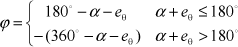
φ = {\begin{matrix} 180^{\circ} - α - e_{θ} & α + e_{θ} \leq 180^{\circ} \\ - (360^{\circ} - α - e_{θ}) & α + e_{θ} > 180^{\circ} \end{matrix}

(1)

If ϕ >0, the AGV stops at the intersection first and then turns left. If ϕ <0, it also stops first and then turns right. If ϕ=0, it can go through the crossroads directly without needing to stop. When the AGV revolves, the actual angle of the turnaround is continually detected by accumulating the pulse signals of two encoders attached to the driving wheels. When the actual value achieves the target value, it stops at the crossing point immediately, and its heading turns to its next pathway given by the routing table. Lastly, the AGV restarts again to follow the new guide-path and departs from the crossroads.

It can be seen that measuring the pose deviations of the AGV and recognizing the multi-branch pattern of the crossroads are the two main tasks of the vision guidance. The former involves measuring geometric dimensions based on vector graphs, a task which can be classed as machine vision, and the latter is the extraction and recognition of features of shape, which can be classed as computer vision. The following parts of the paper focus on the latter. The layout constraints of the vision sensor in the process of crossroads recognition are discussed first. As a result of the vertical downward installation of the on-board camera, the AGV can move in both directions on the guide-paths. Its advantages are obvious, e.g., it can take a shortcut to reduce the travel distance, or resolve a head-on conflict (two AGVs following the same pathway in opposite directions) by withdrawing an AGV. However, its main problem is the scope limitation of its visual field, as shown in Figure 8. Let us assume the image resolution is M×N, the rate of the image sampling is f_c frame/second, and the proportional factor of the physical coordinates to the image coordinates is A_pix pixel/mm. In order to avoid the possibility of the AGV missing the intersection, any landmark on the floor is required to appear in at least n_min successive frames of the images. The maximum speed of the AGV is

v_{\max} = \frac{M f_{c}}{A_{p i x} n_{\min}}

(2)

Figure 8.

Crossroads in the visual field

If the bidirectional AGV cannot recognize the crossroads and choose its next guide-path by the time of n_min /2 frames, it may miss the intersection and even get lost. A_pix means the accuracy of the vision measurement. n_min has a direct impact on the reliability of vision recognition. Increasing M, N and f_c will burden the computing load of image processing and improve the requirements of real-time performance. It can be seen that the AGV's speed and the reliability, accuracy and real-time performance of vision processing are constrained by each other.

The vision sampling process is performed in a continuous time series. When an AGV moves from a guide-path to a T-shaped intersection, the landmark image changes in the visual field, as shown in Figure 9. At the time of frame 1, the forward pathway does not appear in the visual field, and the features of the shapes of the intersection are incomplete, so the vision system cannot identify the T-shaped intersection correctly. Only a small interval of time, after the forward pathway enters the visual field and before the current pathway disappears, is provided for the vision system to recognize the crossroads. In this sense, its reliability and real-time performance are both indispensable.

Figure 9.

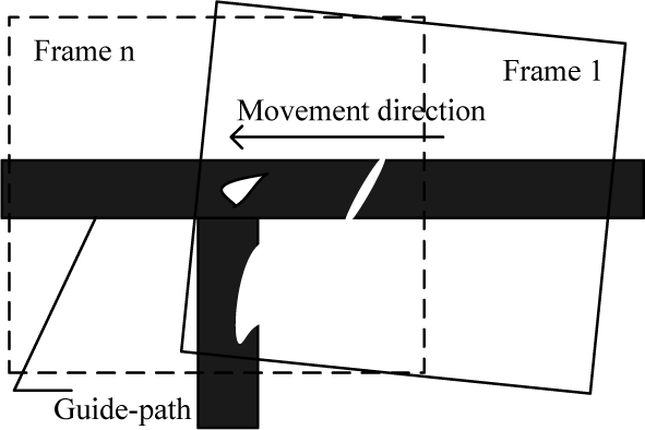
Vision sampling when an AGV enters an intersection

4. Multi-branch intersection recognition

The following operations are usually carried out to identify the object's shapes. Firstly, the features of shapes of the objects are extracted. Then, these objects are classified into different patterns in terms of their features. If the data structure of the features is too complex, it may be necessary to simplify the structure before carrying out the pattern recognition.

4.1 Feature extraction

Features of shapes may be global or local, and their extraction techniques can be contour-based or region-based [23]. The strict requirements on the results of image segmentation limit the applications of contour-based shape description methods [24]. More than 40 techniques for extracting features of shapes are summarized and compared in [25], where the region-based area function is considered not susceptible to covering, distortion and other noises in partial images, and is considered as simple and efficient for use with regular shapes.

Since the object size is relatively small in many cases of shape recognition, the invariance of pan, rotation and zoom is required for feature extraction [26]. However, the intersection of vision guidance has a relatively large size, and the crossroads type will change if the landmark is rotated by more than 90° [27]. The images of the same landmark may have obvious changes when sampled by the AGV at different poses. Besides, many interferences of breakage, contamination, covering and reflecting exist on the actual guide-paths, resulting in region-based features with holes, disconnections and deformities, or incomplete contour-based features, as shown in Figure 9. It is often difficult to repair the randomly-deformed guide-paths by using morphologic algorithms of image processing [25]. Checking sampled rows [14] or matching templates [15] may create a large possibility for misjudging landmarks. In order to avoid this risk, a technique of feature extraction combining region projection and contour scanning is used here for the pattern recognition of crossroads as well as the geometric measurement of deviations.

The digital signal decoded from a PAL analogue video of an on-board camera is in an 8bit YCbCr format of colour images. Cb and Cr are blue and red chrominance components that do not contain luminance. A binary image with a resolution of M×N is obtained after the colour segmentation and filtering in which the image of the tapes is saved but that of the RFID tags is removed. Assume the pixel value is f (i, j), where it is 1 for the landmark and 0 for the background. Scan all the pixels in the row j (1 ≤ j ≤ N) from left to right. Record the first pixel whose value is 1 as hl_j, the last pixel whose value is 1 as hr_j, and the number of pixels whose value is 1 as hp_j. Scan all the pixels in column j (1 ≤ j ≤M) from top to bottom. Record the first pixel whose value is 1 as vt_i, the last pixel whose value is 1 as vb_i, and the number of pixels whose value is 1 as vp_i. In order to measure geometric dimensions based on vector-graphs, the feature point sets by four- boundary contour scanning are

H_{l} = {(x, y) | x = h_{l j}, y = j, j = 1, 2 \cdot \cdot \cdot N}

(3)

H_{r} = {(x, y) | x = h_{r j}, y = j, j = 1, 2 \cdot \cdot \cdot N}

(4)

V_{t} = {(x, y) | x = i, y = v_{t i}, i = 1, 2 \cdot \cdot \cdot M}

(5)

V_{b} = {(x, y) | x = i, y = v_{b i}, i = 1, 2 \cdot \cdot \cdot M}

(6)

In order to recognize the intersection pattern, the region features of landmarks are described by using projection vectors in the directions of row and column, shown as

H_{p} = [\begin{matrix} h p_{1} & \dots & h p_{N} \end{matrix}]

(7)

V_{p} = [\begin{matrix} v p_{1} & \dots & v p_{M} \end{matrix}]

(8)

4.2 Dimensionality reduction

Insert all elements of V_p sequentially behind the end of H_p to constitute a feature vector, P, of M + N dimensions, which describes the global region-based features but has redundant information. In order to search for the significant information in the high-dimensional observational data, the high-dimension vector, P, needs to be projected to a low-dimensional space [28]. Linear discriminant analysis (LDA) is a linear supervised approach for dimensionality reduction . An optimal projection space can be found, in which when the high-dimensional data is mapped, the resulting low-dimensional data of the same classification gather together, and that data of different classifications remain scattered [29]. Assume input samples X belonging to C classifications, and adopt them as a training set. The projection direction matrix W of the LDA is designed for the purpose of minimizing traces of intra-class divergence matrix, S_w, and maximizing that of inter-class divergence matrix, S_b, at the same time [30], shown as

a r g \underset{W}{\begin{matrix}  \end{matrix} m a x} \begin{matrix}  \end{matrix} \frac{t r (W^{T} S_{b} W)}{t r (W^{T} S_{w} W)} s . t . W_{}^{T} W_{} = I_{d}

(9)

S_{w} = \sum_{i=1}^{C} \sum_{j = 1}^{N_{i}} ({\bar{x}}_{j}^{(i)} - {\bar{m}}^{(i)}) {({\bar{x}}_{j}^{(i)} - {\bar{m}}^{(i)})}^{T}

(10)

S_{b} = \sum_{i = 1}^{C} N_{i} ({\bar{m}}_{}^{(i)} - \bar{m}) {({\bar{m}}_{}^{(i)} - \bar{m})}^{T}

(11)

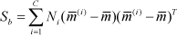
Where N_j is the number of input samples of the i-th classification, ${\bar{x}}_{j}^{(i)}$ is the j-th sample belonging to the i-th classification, m⁻⁽ⁱ⁾ is the mass centre of the i-th classification and ̄ is the mass centre of all the classifications. The generalized eigenvalue approach is used to obtain the projection direction matrix W, shown as

S_{b} w = λ S_{w} w

(12)

When S_w is non-singular, the basis vectors obtained from Eq.(12) correspond to the most important m eigenvectors of S_w⁻¹S_b. The upper limit of m is C −1. Assume the space after dimensionality reduction as Y . For the input samples of C classifications, the dimensionality of space Y is no more than C −1 by using LDA. The resulting vector after dimensionality reduction is

Y = X W

(13)

As shown in Figure 4 and Table 1, there are six types of intersection shapes for crossroads. If we take the shape of the guide- path into account, the total number of landmark classifications should be seven, as shown in Table 3. In order to provide a sampling set for training, 280 pieces of images are collected for each type of landmark (N_j =280). The total capacity of input samples is 1,960.

Table 3.

Landmark pattern definition

Class ID	C1	C2	C3
Landmark	Guide-path	L-shape (a)	T-shape (d)
C4	C5	C6	C7
T-shape (c)	Cross shape	L-shape (b)	T-shape (e)

Let the high-dimension (M + N) feature vector extracted from each image be P_i^C, where C (C =1,2,…7) is the ID of the landmark classification, and i (i =1,2, …280) is the ID of the landmark sample. The dimensionality of feature vector P_i^C is reduced by using LDA. Based on Eq.(9) to Eq.(12), we can obtain the projection direction matrix W_P. By using Eq.(13) we obtain the simplified six-dimension vector X_Pi^C. The first three elements of X_Pi^C are projected into a three-dimensional space, as shown in Figure 10. It can be seen that Class 1 (C1) is separable linearly from Class 2 (C2), Class 3 (C3), Class 3 (C3), Class 4 (C4), Class 5 (C5), Class 6 (C6) and Class 7 (C7), but C2 and C3 gather together closely, and the same situation exists between C4 and C5, and also between C6 and C7.

Figure 10.

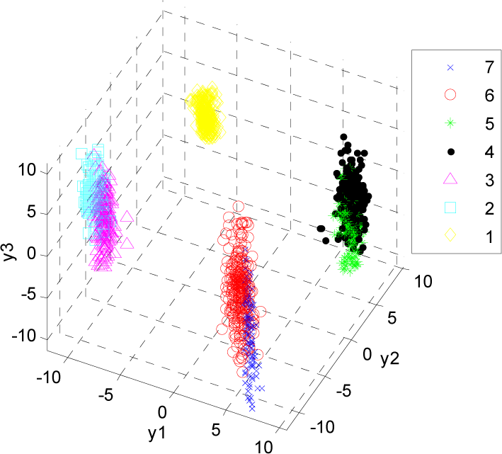
Distribution of the three-dimensional feature vectors after LDA-based dimensionality reduction

4.3 Pattern recognition

Support vector machine (SVM) is a pattern recognition technique suitable for two-classification problems. The kernel trick is used to map the original samples to a high-dimension space, in which a hyperplane that can divide two classifications at the maximum interval is sought. The hyperplane is determined by the training samples on the boundary, and these samples are called support vectors. Assume the sample set is

S = {(x_{i}, y_{i}) | x_{i} \in R^{n}, y_{i} \in {- 1, 1}, i = 1, 2, \dots, I}

(14)

The linear equation of the hyperplane in the n-dimension Euclidean space is

〈 w, x 〉 + b = 0

(15)

Where w is the weighted vector, x is the n-dimension feature vector, 〈w, x〉 is the inner product, and b is the offset vector. The distance of point x to the hyperplane L in that space is

d (x_{i}, L) = \frac{| 〈 w, x_{i} 〉 + b |}{‖ w ‖}

(16)

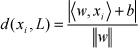
Where ||.|| is the Euclidean 2-norm. The maximization of d(x_i,L) is equivalent to the minimization of ||w||² /2. In this sense, the optimization of the hyperplane can be described as an extreme value problem under constraints, shown as

{\begin{matrix} \min \frac{1}{2} {‖ w ‖}^{2} \\ \begin{matrix} y_{i} (〈 w, x_{i} 〉 + b) \geq 1 & i = 1, 2, \dots, I \end{matrix} \end{matrix}

(17)

Introduce the Lagrange multiplier α = (α₁,α₁,⃛,α_I) α_i ≥ 0 . Construct the dual function of Lagrange as

Q (α) = \sum_{i = 1}^{I} α_{i} - \frac{1}{2} \sum_{i, j = 1}^{I} α_{i} α_{j} y_{i} y_{j} 〈 x_{i}, x_{j} 〉

(18)

Its constraint condition is

\sum_{i, j = 1}^{I} α_{i} y_{i} = 0, α_{i} \geq 0, i = 1, 2, …, I

(19)

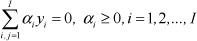
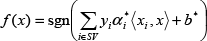
The solution of the dual convex quadratic programming that makes Q(α) maximum is signed as α* = (α*₁, α*₂, ⃛,a*_I). Many components of α* are 0. The samples corresponding to α* >0 are called support vectors SV. The optimal weighted vector and offset vector are

{\begin{matrix} w^{*} = \sum_{j = 1}^{I} α_{j}^{*} y_{j} x_{j} \\ b^{*} = y_{i} - \sum_{j = 1}^{I} y_{j} α_{j}^{*} 〈 x_{j}, x_{i} 〉 \end{matrix}

(20)

Where the samples with the subscript, j, are the support vectors, SV. The optimal classification function suitable for two-class problems is

f (x) = sgn (\sum_{i \in S V} y_{i} α_{i}^{*} 〈 x_{i}, x 〉 + b^{*})

(21)

However, vision guidance in our application needs seven types of landmarks. Constructing an integrated classifier containing several conventional two-class SVMs is an effective approach to handling multi-classification problems [31]. Common construction techniques include One Versus One (OVO), One Versus Rest (OVR) and Binary Tree (BT) [32]. In order to improve the correct rate of recognition, the classifier with the maximum separation interval should be given priority on the top layer. The layer partition is based on the similarity between classes, which can be measured by an intra-class divergence factor

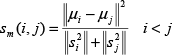
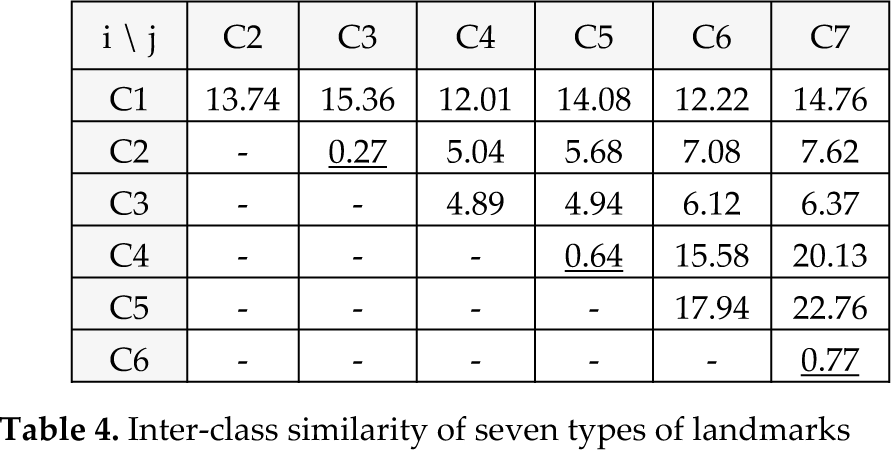
\begin{matrix} s_{m} (i, j) = \frac{{‖ μ_{i} - μ_{j} ‖}^{2}}{‖ s_{i}^{2} ‖ + ‖ s_{j}^{2} ‖} & i < j \end{matrix}

(22)

Where S_i² and S_j² are the square deviations of all the samples of class j and class j, u_i and u_j are the mass centre of class and class j . This factor s_m (i, j) is smaller than 1 when class has similar features to class j . The similarity between each type of landmark is calculated by taking the corresponding vector X_Pi^C to Eq.(22), the result of which is shown in Table 4. It can be seen that the factors between C2 and C3, between C4 and C5, and between C6 and C7 are all smaller than 1, which provides the same classification result as with that in Figure 10. C2, C4 and C6 have similar features to C3, C5 and C7, respectively.

Table 4.

Inter-class similarity of seven types of landmarks

i \ j	C2	C3	C4	C5	C6	C7
C1	13.74	15.36	12.01	14.08	12.22	14.76
C2	-	0.27	5.04	5.68	7.08	7.62
C3	-	-	4.89	4.94	6.12	6.37
C4	-	-	-	0.64	15.58	20.13
C5	-	-	-	-	17.94	22.76
C6	-	-	-	-	-	0.77

Let us have a look at the definition of the landmark pattern in Table 3 and the vision sampling process in the continuous time series in Figure 9. When the T-shaped intersection has just entered the visual field, the features of the shapes of the landmark are temporarily incomplete. As a result, whether the forward pathway exists is unpredictable. If the classes with incomplete features are mapped into a high-dimension space by using the kernel trick to separate them, the generalizability of the classifier may be impaired. In order to improve the real-time performance of the system, a two-layer classifier of SVM is proposed here. The first layer is used for early warning, which quickly judges whether a crossroads is entering the visual field. The second layer is used for decision making, which identifies the type of intersections after whether the forward pathway exists can be judged by the continuous movement of the AGV. The layer-partition rules of the hierarchical SVM classifier are based on a rough set. It is a tool suitable for processing and analysing imprecise, uncertain and indiscernible information and knowledge [33]. Attribute reduction, rule acquisition and intelligent computing are its common applications in the field of machine learning and pattern recognition [34, 35].

From the perspective of a rough set, the training samples of landmarks are regarded as the object set, U, the region projection vectors H_p and V_p are used as two condition attributes, and seven types of landmark pattern are used as decision attributes. A two-layer decision-making table is built for the recognition of landmark patterns, as shown in Table 5. The clustering classification method is utilized to select several similar classes to generate an equivalence class in the rough set. C2 and C3, which both have a left pathway, merge into the equivalence class C23. C4 and C5, with left and right pathways, merge into C45. C6 and C7, with right pathways, merge into C67. C1, C23, C45 and C67 make up layer 1 with the condition attributes of the row projection vector H_p .C2, C4 and C6, without a forward pathway, and C3, C5 and C7 with a forward pathway, merge into two equivalence classes C246 and C357, respectively, on layer 2 with the condition attributes of the column projection vector, V_p. By regulating the granularity of the data, this knowledge learning mechanism transforms a linearly indiscernible problem into a series of linearly discernible problems, so the generalizability of the data and the classification speed of SVM are improved.

Table 5.

Two-layer decision-making table

Layer 1: Object set \ Attributes	Hp	d
U11	1	{C1}
U12	2	{C2,C3}
U13	3	{C4,C5}
U14	4	{C6,C7}
Layer 2: Object set \ Attributes	Vp	d1
U21∪U22∪U23	1	{C2,C4,C6}
U21∪U22∪U23	2	{C3,C5,C7}

In order to deal with the incomplete features of shapes when a landmark has just entered the visual field, a security zone is divided from the whole visual field to ensure correct decision-making in landmark classification.

It is combined with the two-layer decision-making table to form a hierarchical SVM classifier for landmark recognition, as shown in Figure 11. On the first layer of early warning, C1, C23, C45 and C67 need to be separated from each other. LDA is used to reduce the dimensionality of the row and the column projection vectors H _Pi ^C and V _Pi ^C , which are converted to the three-dimensional projection vectors ¹X_Hi^C and ¹X_Vi^C. Their first two dimensions are projected as shown in Figure 12. Landmark samples are divided into four separate classes, C1, C23, C45 and C67, according to the three-dimension feature vector, ¹X_Hi^C. Since all the original samples are already linearly separable, the technique of constructing OVO is used for the four-classification problem. Six linear SVMs are designed to find a hyperplane with the maximum interval between each two classes.

Figure 11.

Hierarchical SVM classifier for landmarks

Figure 12.

The first two-dimension projection on the early warning layer

The classification decision function is

\begin{matrix} f (x_{i j}) = sgn (w_{i j}^{*} x + b_{i j}^{*}) & 1 \leq i < j \leq 4 \end{matrix}

(23)

Where the optimal weighted vector w*_ij and offset vector b*_ij can be computed by using Eq. (20). The sample to be recognized is brought into the six SVM sub-classifiers described by Eq.(23). Add the judgment result of each sub-classifier to the count of the corresponding class, and the resulting class is that which has the highest count.

On the second layer of decision making, C246 and C357 create a two-classification problem that actually reflects whether the forward pathway exists. LDA is used to reduce the dimensionality of the row and column projection vectors H _Pi ^C and V _Pi ^C again. The projection of the training samples are one-dimension points ²X_Hi^C and ²X_Vi^C, as shown in Figure 13. Landmark samples cluster in an intensive line segment. C246 cannot be separated from C357 regardless of whichever one-dimensional feature parameter ²X_Hi^C and ²X_Vi^C is used. However, the sample distribution of ²X_Vi^C is relatively more scattered than that of ²X_Hi^C, so ²X_Vi^C is adopted as the classification basis on this layer.

Figure 13.

The one-dimension projection on the decision making layer

A security zone is defined to ensure the correct classification decision is made once the landmark in the visual field already has the complete features of the shapes. The SVM classifier does not check temporarily whether the forward pathway exists when the crossing point is located in the beginning and end area of the Sa pixels in the visual field. The symmetrical area of M − 2Sa pixels around the centre of the AGV, O_A, is relatively secure for classification decisions, as shown in Figure 14. With the increase of the secure distance, Sa, the reliability of identifying the landmark classification is improved, but the time left for processing and analysing the landmark image is reduced.

Figure 14.

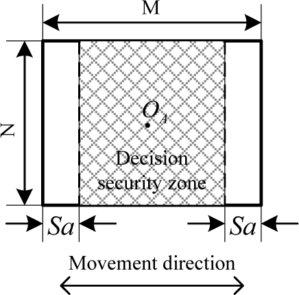
Definition of decision security zone

The machine learning algorithm is applied to the column feature parameter, ²X_Vi^C, to find the relation between the secure distance, Sa, and the misjudgment probability and the classification interval (that is the distance between the two nearest points which belong to two different types of samples). It is a regression process that gradually eliminates the training samples according to its degree of proximity to the column boundary, from both ends of the column to its midpoint until it finds an area in which two types of samples are separated from each other. As shown in Figure 15, with the increase of the secure distance, Sa, by a step value of 15 pixels, the column feature parameter, ²X_Vi^C, of two types of training samples are gradually divided into two isolated plots, which means that two types of samples are linearly separable in the security area.

Figure 15.

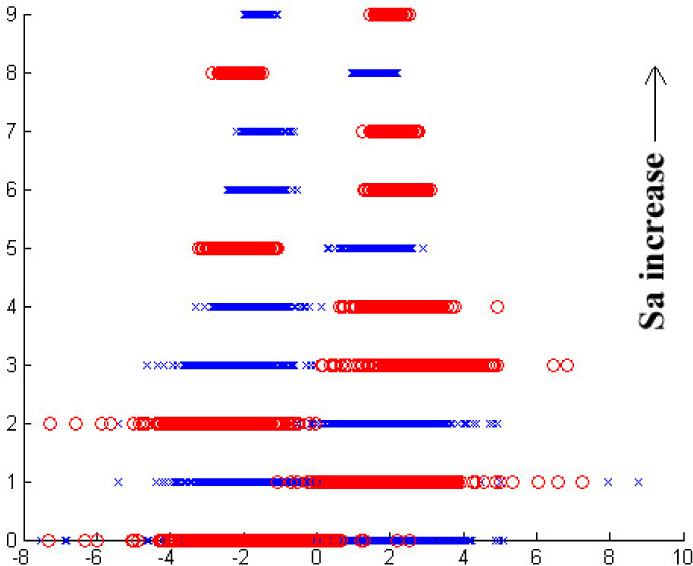
Distribution of samples in the security zone

Figure 16 shows the changes in the misjudgment probability and classification interval when two types of samples are recognized by using different secure distances. Generally, the decision security zone can be delineated by the secure distance, the misjudgment probability of which is zero. When considering possible errors presented by a finite number of samples, it is more reliable to add a proper margin to the value of secure distance. It is seen that the misjudgment probability is 0 when the secure distance is 108. Add a margin of 50% to this value, and set the secure distance as Sa =162. At this time, the classification interval is 0.832.

Figure 16.

Misjudgment probability and classification interval in the security zone

5. Experiment and discussion

A low-cost vision guidance system is developed by using commercial off-the-shelf components, such as an on-board camera with a 3.5-8mm manual zoom lens, a LED ring light, a digital signal processor (DSP) TMS320DM642 for image processing and an advanced RISC machine (ARM) LPC2292 to control the AGV. A three-phase agent-oriented design approach is used for the development of a control system which has the multitasking processing capacity owing to multiple microprocessors and system services of RTOS [19]. The on-board camera has an image resolution of 720 ×576 pixels and a sample rate of 25 frames/s. The proportional factor A_pix between the physical coordinates and the image coordinates is estimated at 2.0656 pixel /mm by calibrating the vision system. Assuming the maximum speed of the AGV is 1m/s, the distance of two positions of one image point appearing in two consecutive frames is 82.6 pixels. The secure distance, Sa, from the security zone to the column boundaries of the visual field is 162 pixels. The vision system can make a correct classification decision in the second frame when the intersection enters the visual field. Each scene point appears in at least 8.7 frames of the images at the maximum speed, according to Eq.(2). It can be seen that there is a high margin of safety for crossroads classification.

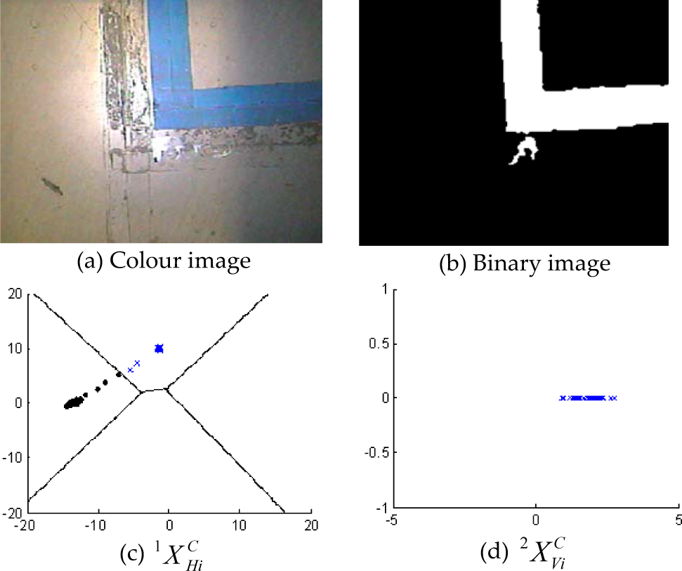
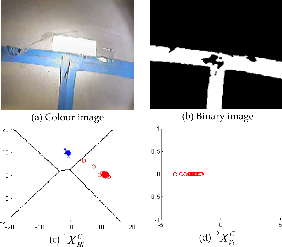
In our experiment, L-shaped, T-shaped and cross-shaped intersections are all tested on a floor of different materials, a concrete floor or a terrazzo floor, to check the possible effects of the floor on the recognition technique. Figure 17, 18, 19 and 20 shows the recognition results of the L-shaped right-turning crossroads (C6), the L-shaped left-turning crossroads (C2), the T-shaped left/forward-turning crossroads (C3) and the cross-shaped crossroads (C5). Figure 17 and 19 are used for the test on the concrete floor, and Figure 18 and 20 are used for the terrazzo floor. The colour images of the four types of intersections are shown in Figure 17.(a), 18.(a), 19.(a) and 20.(a), and their binary images are shown in Figure 17.(b), 18.(b), 19.(b) and 20.(b). On the first layer of the hierarchical SVM classifier, the high-dimension row projection vectors, H _Pi ^C , are simplified to three-dimension feature vectors, ¹X_Hi^C, by using LDA. The projection of their first two dimensions is shown as the feature points in Figure 17.(c), 18.(c), 19.(c) and 20.(c). Only in the state transition process when the intersection just enters the visual field of AGV, are the feature points located close to the boundary of guide-path class (C1), and at other times these points maintain a relatively large secure distance from the boundary. It illustrates that the first layer of the classifier can make a correct decision after the state transition process.

Figure 17.

Recognition results of L-shape right-turning crossroads on the concrete floor

Figure 18.

Recognition results of L-shape left-turning crossroads on the terrazzo floor

Figure 19.

Recognition results of T-shape left/forward-turning crossroads on the concrete floor

Figure 20.

Recognition results of cross-shape crossroads on the terrazzo floor

On the second layer of the hierarchical SVM classifier, the high-dimension column projection vectors, V _Pi ^C , are simplified to one-dimension feature points, ²X_Vi^C, as shown in Figure 17.(d), 18.(d), 19.(d) and 20.(d). The feature points are distributed away from the boundary of the other class, which illustrates that the second layer of the classifier does not misjudge landmarks when the intersections arrive in the security zone of the classification decisions. In order to further improve the reliability of the classification decisions, only the SVM classifier obtains the same recognition results for two consecutive frames of images, the DSP sends this result to the ARM that controls the AGV's movement through the crossroads. Figure 17.(b) shows that the visual noises caused by the contaminated spots outside the landmarks do not interfere with the recognition results of the SVM classifier. Figure 19.(b) and 20.(b) show that the SVM classifier is not sensitive to the breakages on the edge of the guide-paths and the holes inside. Figure 17.(a), 18.(a), 19.(a) and 20.(a) show that the change of floor materials has no effect on the recognition results. All of the above verify the reliability and robustness of our vision recognition technique.

In order to test the performance of the AGV navigation in a bidirectional flow network, we construct a complex fixed-path map with branches and nodes on the terrazzo floor by using blue adhesive taps and RFID tags, according to the topology structure as shown in Figure 2. There are six guide-paths (denoted a to f), two crossroads (denoted 3 and 4) and four workstations (denoted 1, 2, 5, 6), which form a unidirectional closed-loop guide-path (a-b-c) and two bidirectional open-loop guide-paths (d and e-f). The routing table is automatically generated for each of the two nodes by using a path planning technique according to the adjacent matrix of its topological map in the central computer on the system design stage, as shown in Table 2. This table is downloaded to the on-board controller of all the AGVs before the whole system runs. The topological data of two crossroads (node 3 and 4) stored in the intersection tags are as follows.

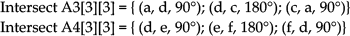
\begin{array}{l} Intersect A3[3] [3] = {(a, d, 90°); (d, c, 180°); (c, a, 90°)} \\ Intersect A4[3] [3] = {(d, e, 90°); (e, f, 180°); (f, d, 90°)} \end{array}

At the stage of operating the system, when the AGV receives a transportation task, it can know its target node. As long as it reads a milestone tag or intersection tag or station tag, it can know its current absolute location in the global map. When it arrives at the exit end of a pathway, it can read a pathway tag and know whether the next node is a crossroads. If it is a crossroads, the AGV can select the next pathway according to the routing table, and read the local topological relation from an intersection tag. A searching algorithm is used to compute the angle of the turnaround according to Eq.(1) by the on-board controller of the AGV. Then the AGV stops at the crossing point, turns around its centre by the target angle, and re-orientates its heading to the new pathway. We use a digital camera (not mounted on the AGV) and record its typical positions and actions in the bidirectional flow network, as shown in Figure 21.

Figure 21.

Typical positions and actions of the AGV in intelligent navigation experiments

Task 1 is to travel from workstation 2 to workstation 1. The AGV leaves node 2 and first arrives at a left-turning crossroads (it is not denoted as a node since there is only one next possible pathway) on pathway c (shown as Figure 21.(a)). The hierarchical SVM classifier on the DSP recognizes the landmark as C2, and sends the result to the ARM, which controls the AGV, making it turn left around the corner (shown as Figure 21.(b)). Then the AGV continues to follow another section of pathway c until it arrives at intersection 3 (shown as Figure 21.(c)). According to its current location (node 3) and the destination (node 1), its next node (node 1) and pathway (a) is selected by using the routing table. The SVM classifier recognizes the T-shaped crossroads as C3, which matches the topological information of array A3 obtained from the intersection tag. The target angle of the turnaround is ϕ =90° according to Eq.(1), so the AGV turns left 90° around intersection 3 (shown as Figure 21.(d)), and changes its heading from pathway c to pathway a (shown as Figure 21.(e)). Then it continues to follow the new pathway until it arrives at workstation 1.

Task 2 is to travel from workstation 2 to workstation 5. When the AGV arrives at intersection 3, the target angle of the turnaround is 0°, according to Eq.(1), so it continues to follow pathway c until it goes through the crossroads and enters pathway d (shown as Figure 21.(f)). When it arrives at intersection 4, the target angle of the turnaround is 90°, so it stops at the crossing point first and then turns left (shown as Figure 21.(g)). Then it continues to follow pathway e until it gets to its destination.

Task 3 is to travel from workstation 5 to workstation 6. When the AGV arrives at workstation 5 on the endpoint of pathway e, it rotates 180° clockwise around that point (shown as Figure 21.(h) and 21.(i)) and changes its heading direction to be back to workstation 6 (shown as Figure 21.(j)). Then it comes back along the same pathway e until it gets to intersection 4. Since the target angle of the turnaround is 0°, according to Eq.(1), the AGV goes through intersection 4 directly and follows pathway f (shown as Figure 21.(k)) until it reaches the other endpoint. The same turning back occurs at workstation 6 and the AGV is again heading to workstation 5 (shown as Figure 21.(l)). It is seen that the AGV can travel along pathway e and f in both directions, and hence they are bidirectional.

Task 4 is to travel from workstation 5 to workstation 1. When the AGV travels along pathway e (shown as Figure 21.(m)) and gets to intersection 4, the target angle is −90° according to Eq.(1), so it turns right to change its route to pathway d (shown as Figure 21.(n)). Then it continues to follow this pathway (shown as Figure 21.(o)) until it finds intersection 3. Since the target angle of the turnaround is − 90°, the AGV turns right to enter pathway a (shown as Figure 21.(p)). Then it departs from intersection 3 to workstation 1. It can be seen that pathway d is bidirectional, but pathways 1, 2 and 3 are all unidirectional.

Figure 21 shows that there are intensive illumination reflections and inverted images on the floor. The vision guidance system of our AGV can still recognize different landmarks accurately and reliably without being disturbed by image noises from its surroundings, and the on-board controller can make the vehicle complete a series of intelligent actions according to its electronic map in the bidirectional flow network.

6. Conclusion

Owing to its motion freedom to deviate from guide-paths, a free-ranging AGV is often considered as more adaptable and intelligent than a line-tracking AGV on fixed paths. Fixed paths indeed imply motion constraints that prevent an AGV from moving freely. However, for a large number of AGVs, although these constraints bring inconveniences to a single AGV, they may at the same time set potential rules for coordinating the individual movements of AGVs and to reduce space-seizing conflicts especially when many AGVs cluster in finite-space environments. Besides, there are many fruitful design methodologies for AGV transportation systems for fixed-path guidance, and equipment expense is also an important factor to be considered when many large-scale AGV systems are constructed. It is very useful to develop a smart AGV that can attain high flexibility while retaining low-cost, simplicity and reliability on fixed paths.

Visible tapes and RFID tags are used to install a navigation infrastructure on the floor. The former can describe features of shapes and geometric dimensions of intersections and lines, and the latter can directly record global locations on pathways and the local topological relations of crossroads. A topological map is easy to build and edit on a central computer, in which all the elements of nodes, pathways and crossroads only need schematic signs rather than accurate poses when establishing a priori knowledge of the workplace. The routing table is stored in the on-board controller as a simplified form of topological map. The AGV has a high degree of on-board autonomy, including being able to locate itself on guide-paths precisely, recognizing different multi-branch crossroads intelligently by verifying the conformance of vision and RFID information, and selecting its next pathway efficiently.

The on-board camera is mounted downward vertically on the centre of the AGV in order to guide it in both directions. The small visual field provides great difficulty for vision-based recognition and measuring for landmarks in factories, especially for multi-branch intersections. First, the methods of region projection and contour scanning are both used to extract the features of the shapes of intersections. Then LDA is used to reduce the number of the dimensions of features. Third, a hierarchical SVM classifier is proposed to classify different multi-branch patterns when the AGV enters the security zone in which the landmark has the complete features of shapes. The experiments for vision recognition show that our low-cost vision guidance system is insusceptible to visual noises, image breakages and floor changes. The recognition technique can work effectively in real-time, whilst providing the repeatability and reliability needed in industry. The vision-based AGV can travel on optimal routes, pass through different crossroads and arrive at its destination intelligently in a bidirectional flow network.

Modern techniques of vision recognition and RFID perception have improved the navigation intelligence of low-cost AGVs to some extent. However, their localization and guidance are still dependent on artificial landmarks, and hence these AGVs are restricted to guide-paths without the ability to deviate from these fixed paths even if their paths are occluded by some uncontrollable obstacles. They have to stop at their spots at that moment in order to avoid collisions and to wait for manual operation. Future research could involve looking into local free-ranging navigation that can permit an AGV to deviate from guide-paths temporarily in order to bypass the occluded spots. Other on-board cameras may be necessary in order to look forward with a larger and deeper visual field. The local position and orientation can be estimated by using a neural extended Kalman filter in a monocular visual SLAM framework [8]. The projection region size of the obstacle can be estimated based on worst-case avoidance conditions and the virtual force field-based algorithm can be used for avoiding moving obstacles [36]. If the low-cost vision-based AGVs have the intelligence of local real-time SLAM and autonomous obstacle avoidance, this will be helpful in convincing industrial practitioners of the virtues of vision navigation, and to promote the further application of vision-based AGVs in more large-scale AGV systems that may require flexibility, simplicity, efficiency and low cost at the same time.

7. Acknowledgments

This research is supported by the National Natural Science Foundation of China (No.61105114 and No.51175262), the Natural Science Foundation of Jiangsu Province of China (BK201210111), and the Priority Academic Program Development of Jiangsu Higher Education Institutions (PAPD).

References

Le-Anh

De Koster

M.B.M.

A review of design and control of automated guided vehicle systems. Eur. J. Oper. Res., 2006, 171(1): 1–23.

Iris

F.A. Vis

Survey of research in the design and control of automated guided vehicle systems. Eur. J. Oper. Res., 2006, 170(3): 677–709.

Martínez-Barberá

Humberto

Herrero-Pérez

David

Autonomous navigation of an automated guided vehicle in industrial environments. Robot. Comput. Integr. Manuf., 2010, 26(4): 296–311.

Herrero-Pérez

David

José

Juan

Alcaraz-Jiménez Martínez-Barberá

Humberto

An accurate and robust flexible guidance system for indoor industrial environments. Int. J. Adv. Robot. Syst., 2013, 10(292): 1–10.

Kelly

Alonzo

Nagy

Bryan

Stager

David

An infrastructure-free automated guided vehicle based on computer vision. IEEE Robotics & Automation Magazine, 2007, 14(3): 24–34.

Civera

Davison

A.J.

Montiel

J.M.M.

Inverse depth parametrization for monocular SLAM. IEEE Trans. Robot, 2008, 24(5): 932–945.

Paz

L.M.

Pinies

Tardos

J.D.

Neira

Large scale 6DOF SLAM with stereo-in-hand. 2008, IEEE Trans. Robot, 24(5): 946–957.

Miljkoviæ

Zoran

Vukoviæ

Najdan

Mitiæ

Marko

New hybrid vision-based control approach for automated guided vehicles. Int. J. Adv. Manuf. Technol., 2013, 66: 231–249.

Beccari

Caselli

Zanichelli

Vision-based line tracking and navigation in structured environments. In: Proc. of the IEEE Int. Symp. on computational intelligence in robotics and automation, USA, 1997: 406–411.

10.

Rodriguez

F.J.

Mazo

Sotelo

M.A.

Automation of an industrial fork lift truck, guided by artificial vision in open environments. Auton. Robot., 1998, 5: 215–231.

11.

Park

Lee

J-W

Vision-based AGV parking system. J. Inst. Control Rob. Syst., 2009, 15(5): 473–479.

12.

Baglivo

Biasi

Biral

Autonomous pallet localization and picking for industrial forklifts: a robust range and look method. Meas. Sci. Technol., 2011, 22: 085–502.

13.

Seelinger

Yoder

J.D.

Automatic visual guidance of a forklift engaging a pallet. Robot. Auton. Syst., 2006, 54: 1026–1038.

14.

Wang

A study on cross road recognizing for vision-based auto guided vehicle system. Journal of Image and Graphics, 2000, 8(5): 632–637.

15.

Zhang

Yuan

Mei

Visual navigation of an automated guided vehicle based on path recognition. In: Proc. of Int. Conf. on Machine Learning and Cybernetics. Monterey, 2004: 3877–3881.

16.

Chen

Sun

Tracking control of automatic guided vehicle based on lane marked navigation. Chinese Journal of Mechanical Engineering, 2006, 42(8): 164–170.

17.

Park

Hashimoto

An intelligent localization algorithm using read time of RFID system. Adv. Eng. Inf., 2010, 24(4): 490–497.

18.

Zhang

Chen

Precise localization of mobile robots via odometry and wireless sensor network. Int. J. Adv. Rob. Syst., 2013, 10(203): 1–13.

19.

Lou

Agent-oriented embedded control system design and development of a vision-based automated guided vehicle. Int. J. Adv. Robot. Syst., 2012, 9(37): 1–11.

20.

Yoon

H.S.

You

J.O.

Park

T.H.

Dynamic path planning for autonomous mobile robots. J. Inst. Control Rob. Syst., 2008, 14(4): 392–398.

21.

Sathyaraj

B.M.

Jain

L.C.

Finn

Multiple UAVs path planning algorithms: A comparative study. Fuzzy Optim. Decis. Mak., 2008, 7(3): 257–267.

22.

Lou

Tang

Integrated motion control of path tracking and servo control for an automated guided vehicle. Chinese Journal of Mechanical Engineering, 2011, 47(3): 43–48.

23.

Zhang

Review of shape representation and description techniques. Pattern Recogn., 2004, 37(1): 1–19.

24.

Thacker

N.A.

Clark

A.F.

Barron

J.L.

Performance characterization in computer vision: A guide to best practices. Computer vision and image understanding, 2008, 109(3): 305–334.

25.

Yang

Kpalma

Ronsin

J.A.

survey of shape feature extraction techniques. Pattern Recogn., 2008, 41(1): 43–90.

26.

Belongie

Malik

Puzicha

Shape matching and object recognition using shape contexts. IEEE Trans. Pattern Anal. Mach. Intell., 2002, 24(4): 509–522.

27.

Ling

Jacobs

D.W.

Shape classification using the inner-distance [J]. IEEE Trans. Pattern Anal. Mach. Intell., 2007, 29(2): 286–299.

28.

Tenenbaum

J.B.

Silva

V.D.

Langford

J.C.

A global geometric framework for nonlinear dimensionality reduction. Science, 2000, 290(5500): 2319–2323.

29.

A two-stage linear discriminant analysis via QR-decomposition. IEEE Trans. Pattern Anal. Mach. Intell., 2005, 27(6): 929–941.

30.

Nie

Xiang

Liu

Orthogonal vs. uncorrelated least squares discriminant analysis for feature extraction. Pattern Recogn. Lett., 2012, 33(5): 485–491.

31.

Hsu

C.W.

Lin

C.J.

A comparison of methods for multiclass support vector machines. IEEE Trans. Neural Networks, 2002, 13(2): 415–425.

32.

Cheong

S.H.

Lee

S.Y.

Support vector machines with binary tree architecture for multi-class classification. Neural Information Processing Letters and Reviews, 2004(2): 47–51.

33.

Pawlak

Rough set approach to knowledge-based decision support. Eur. J. Oper. Res., 1997, 99(1): 48–57.

34.

Swiniarski

R.W.

Skowron

Rough set methods in feature selection and recognition. Pattern Recogn. Lett., 2003, 24(6): 833–849.

35.

Thangavel

Pethalakshmi

Dimensionality reduction based on rough set theory: A review. Appl. Soft Comput. J. 2009, 9(1): 1–12.

36.

Zeng

Lingqi

Gary

M. Bone.

Mobile robot collision avoidance in human environments. Int. J. Adv. Robot. Syst., 2012, 9: 1–14.

Intersection Recognition and Guide-Path Selection for a Vision-Based AGV in a Bidirectional Flow Network

Abstract

Keywords

1. Introduction

2. System configuration

3. Intelligent navigation framework

4. Multi-branch intersection recognition

4.1 Feature extraction

4.2 Dimensionality reduction

4.3 Pattern recognition

5. Experiment and discussion

6. Conclusion

7. Acknowledgments

References