
Abstract
This paper describes position control of autonomous mobile robot using combination of Kalman filter and Fuzzy logic techniques. Both techniques have been used to fuse information from internal and external sensors to navigate a typical mobile robot in an unknown environment. An obstacle avoidance algorithm utilizing stereo vision technique has been implemented for obstacle detection. The odometry errors due to systematic-errors (such as unequal wheel diameter, the effect of the encoder resolution etc.) and/or non-systematic errors (ground plane, wheel-slip etc.) contribute to various motion control problems of the robot. During the robot moves, whether straight-line and/or arc, create the position and orientation errors which depend on systematic and/or non-systematic odometry errors. The main concern in most of the navigating systems is to achieve the real-time and robustness performances to precisely control the robot movements. The objective of this research is to improve the position and the orientation of robot motion. From the simulation and experiments, we prove that the proposed mobile robot moves from start position to goal position with greater accuracy avoiding obstacles.
Introduction
Autonomous robot navigation is a popular research area which has still many open problems. There are many attempts to solve the problems related to mobile robot navigation in both known and unknown environments. For the mobile robot navigation system, the motion control is importance for robot navigation. Utilizing the odometry data for motion control, (Johann Borenstein, (1998)) has tested a method called the Internal Position Error Correction (IPEC) for detection and correction of odometry error without inertial or external-reference sensors. Other researchers (Hakyoung Chung & Lauro Ojeda & Johann Borenstein, (2001)) have improved the dead-reckoning accuracy with fiber optic gyroscopes (FOGS) using Kalman filter technique that fuses the sensor data from the FOGS with the odometry system of the mobile robot. An Extended Kalman Filter technique is used for building a localization system (Atanas Georgiev & Peter K. Allen, (2004)). This technique integrates the sensor data and keeps track of the uncertainty associated with it. Authors (W.S. Wijesoma; P.P. Khaw & E.K. Teoh, (2001)) have presented a fuzzy behavioral approach for local navigation of an autonomous guided vehicle. Distributed sensor-based control strategy for mobile robot navigation has been proposed by (T.M. Sobh; M. Dekhil, A.A. Efros & R. Mihali, (2001)). Authors (Toshio Fukuda; Fellow & Naoyuki Kubota, (1999)) have focused on a mobile robotic system with a fuzzy controller and proposed a sensory network that allows the robot to perceive its environment. For obstacle avoidance in mobile robot navigation, authors (Alexander Suppes; Frank Suhling & Michael Hotter, (2001)), have proposed an approach using video based obstacle detection for a mobile robot based on probabilistic evaluation of image data. Obstacle detection is realized by computing obstacle probability and subsequent application of a threshold operator. They also identified other types of systematic error and non-systematic error related to the mobile robot's motion such as odometry error due to inadequate encoder resolution, unequal wheel diameter, orientation error due to presence of slippage, angular velocity error of the gyroscope, floor, etc.
The organization of the paper is as follows: section 2 presents a brief description of navigation system of elaborated of fusing together mobile robot developed as part of this research. The proposed approach to solve the robot motion problem is in section 3. In section 4 and 5, we describe the methodology Extended Kalman Filter, Fuzzy Logic Control, and Obstacle Avoidance techniques to implement the proposed system including hardware and software realization. The experimental results are shown in section 6. Conclusion and future research direction are given in section 7.
Mobile robot navigation techniques
The dead-reckoning principle has been used as standard technique navigation for mobile robot positioning. The fundamental idea of dead reckoning is based on a simple mathematical procedure for determining the present location of the robot by advancing previous position through known course and velocity information over a given length of time (H.R. Everett, 1995).
This allows for used of measured wheel revolutions to calculate displacement relative to floor. The advantage of odometry is that it provides good short-term accuracy and allows very high sampling rates.
Kalman Filter
Kalman filter (KF) is widely used in studies of dynamic systems, analysis, estimation, prediction, processing and control. Kalman filter is an optimal solution for the discrete data linear filtering problem. KF is a set of mathematical equations which provide an efficient computational solution to sequential systems. The filter is very powerful in several aspects: It supports estimation of past, present, and future states (prediction), and it can do so even when the precise nature of the modeled system is unknown. The filter is derived by finding the estimator for a linear system, subject to additive white Gaussian noise (Ashraf Aboshosha, 2003). However, the real system is non-linear, Linearization using the approximation technique has been used to handle the non-linear system. This extension of the nonlinear system is called the Extended Kalman Filter (EKF). The general non-linear system and measurement form is as given by equation (1) and (2) as follows:


where xk is a state vector and zk is a measurement vector at the time k, f(·) and z(·)are non-linear system and measurement function, uk is input to the system, wk, γk and vk are the system, input and measurement noises respectively‥ wk ∼ N(0, Q), γk ∼ N(0, Γ) and vk ∼ N(0, R) indicate a Gaussian noise with zero mean and covariance matrix Q, Γ and R (Evgeni Kiriy & Martin Buehler, 2002).
The main operation of Extended Kalman Filter is divided into two parts, the prediction part and the correction part.
Prediction part: This part of the EKF predicts the future state of the system Correction part: This part performs the measurement update using equation (5), (6) and (7) as shown below:
where I is an identity matrix and system (A), input (B), and measurement (H) metrics are calculated by Jacobians of the system f(·) and measurement h(·) (Evgeni Kiriy & Martin Buehler, 2002) using equations (8), (9) and (10).


The idea of fuzzy sets was proposed by Lofti A. Zadeh in July 1964. The Fuzzy Logic can be used for controlling a process (i.e., a plant in control engineering terminology) which is non-linear, the advantage of Fuzzy logic control is that it enables control engineers to easily implement control strategies which can be used by human operator. Its core technique is based on four basic concepts: fuzzy sets, linguistic variables, possibility distributions and fuzzy if-then rule (John Yen & Reza Langari, 1999). Fuzzy logic has been applied to various control system. The block diagram of fuzzy logic controller shown in Fig. 1 is composed of the following four elements (Kevin M. Passino & Stephen Yurkovich, 1998):

The block diagram of fuzzy logic control system
A rule-base (a set of If-Then rules), which contains a fuzzy logic quantification of the expert's linguistic description of how to achieve good control. An inference mechanism (also called “inference engine” or “fuzzy inference” module), which emulates the expert's decision making in interpreting and applying knowledge about how best to control the plant. A fuzzification interface, which converts controller inputs into information that the inference mechanism can easily use to activate and apply rules. A defuzzification interface, which converts the conclusions of the inference mechanism into actual inputs for the process.
The basic idea of a typical stereo vision system is to find corresponding points in stereo images and infer 3D knowledge about the environment. Corresponding points are the projections of a single 3D point in the different image spaces. The difference in the position of the corresponding points in their respective images is called disparity (Marti Gaëtan, 1997). The ideal situation is illustrated in Fig. 2. An arbitrary point in a 3-D scene is projected into different locations in stereo images.

A typical 3-D scene projected in stereo images
Assume that a point P in a surface is projected onto two cameras image planes, PL and PR, respectively. When the imaging geometry is known, the disparity between these two locations provides an estimate of the corresponding 3-D position. Specifically, the location of P can be calculated from the known information, PL and PR, and the internal and external parameters of these two cameras, such as the focal lengths and positions of two cameras. Shown in Fig. 2 is a parallel configuration, where one point, p(x,y,z), is projected onto the left and right of the imaging planes at PL(xl,yl) and PR(xr,yr), respectively. The coordinates of P can be calculated (Jung-Hua Wang & Chih-Ping Hslao, 1999) using equation (11) as follow:

where (xl -xr) is the disparity, base line b is the distance between the left and right cameras, and f is the focal length of the camera
The motion control problem
In most robot's motion, it is very likely that there are positioning problems when the robot moves from a starting position to a goal position. This error may include the orientation error due to slippage during the move.
Assume R to be a robot, this robot starts from an initial position P0 to the goal position Pg in an unknown workspace. Let O be an obstacle in the required workspace W. During a robot move from current position Pk to the next position Pk+1, there is a change in the position and/or orientation. This change causes accuracy problem the robot's location from in calculating current position to next position. The new location is not a verified true position. The position error increases as the robot keeps moving as shown on Fig. 3.

Typical robot move
A mobile robot has been developed in this research, as shown in Fig. 4 and Fig. 14a. It was built on a circular platform with three-wheel configuration. The robot has a diameter of 340 mm and a height of 170 mm. It consists of two driven wheels in the front and single passive wheel in the rear. An optical encoder is mounted on the axis of each wheel used for the odometry measurement.
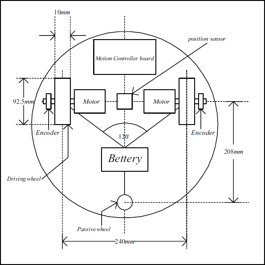
Schematic diagram of the mobile robot
Three separate modules are used external sensors. A vector compass module which is attached to the middle of the robot's chassis to measure the robot heading. A position sensor module which is placed underneath robot chassis 3 mm above the floor to provide the robot position. The last module, the vision sensor is placed on top of the upper circular platform of the mobile robot to provide the stereo vision capability to the robot.
The proposed mobile robot controller is actually a small computer network consisting of an embedded PC (a PC104) and two microcontrollers (DS89C420). All of them are connected together as show in Fig. 5.

Network architecture of the robot
The PC104 is the master controller for the mobile robot, it controls all the activities of two slave controllers (DS89C420s). On a typical robot command, the master controller collects the following information from the Microcontrollers,: optical encoder feedback data from both wheels, robot heading data from vector compass module and absolute position from position sensor module. The slave controllers also act as protocol converters. This eliminates all the protocol conversion burden for the Master controller and allows the PC104 to concentrate only on the necessary control calculations. Table 1. provides typical protocol conversion burden times for each microcontroller.
Typical protocol burden's time between PC104 and Microcontrollers

With this approach, the maximum time for updating the position control command is approximately 8 milliseconds. The motor response time is set at 20 milliseconds interval.
As mentioned before there are 4 sensors mounted on the mobile robot: vector compass, wheel encoder, position sensor and vision sensor.
The detail characteristics of sensors are follows:
Vector compass: this is an electronic compass module with a resolution of 0.1 degree (more resolution is also possible with appropriate hardware and software configurations). Appropriate calibrations techniques provided by the manufacturer cancle out the errors due to variation of the local geomagnetic field and geographic north effects. Wheel encoder: each wheel of the mobile robot is equipped with an optical encoder (with 200 counts per revolution). This allows each axis to provide separate wheel's information independently and accurately. The speed of the motor is set at 50 revolutions per minute, with this speed, the time interval between each encoder pulse is 100 microseconds. Position sensor: this is an electronics sensor based on encoder circuit, to provide direction and counts on 2 linear axes (x-axis and y-axis). The normal resolution is 400 counts/inch (with a maximum resolution of 800 counts/inch). This is an attempt to minimize the computation due to translation during the robot movement. Stereo vision sensor: this is a vision sensor which consists of a two-camera module (The Digiclops™ Stereo Vision camera) to perform range measurements for sensing the environment. It is possible to determine the distance to points in the scene reliably in a range from 0.5 to 6.0 meters.
Fig. 6 shows a block diagram for our proposed motion control system. In the proposed algorithm stereo vision is used to calculate the 3D position of obstacles in the robot path. Extended Kalman Filter, Fuzzy Logic technique and Obstacle avoidance have been implemented in the proposed new motion control system (including information from various sensors). The proposed algorithm has improved the robot's movement as well as the robot's position and orientation.

Block diagram of the proposed motion control system
The operation of the proposed motion control algorithm can be summarized as follows:
Set the start and goal position. Check obstacles in front of the robot using stereo vision sensor. If the robot finds an obstacle, then it computes the avoidance angle or/and the remaining distance to the goal. After the robot has computed the angle error and the distance error in step 2, robot then calculates a set of velocity of the left and the right wheels using the Fuzzy Logic technique. While the robot moves, it verifies a motion's information from the existing internal and external sensors. The Extended Kalman Filter is activated for the robot's motion. If robot does not reach the required goal position, the algorithm step 2 is repeated.
For implementing the proposed system, complete control operation is divided into separate sections. Each section has it's own function. The sections are are: Kinematics Model (a two wheels mobile robot with optical encoders), Fuzzy Logic Control (FLC), the Extended Kalman Filter (EKF) and Obstacle Avoidance. Fuzzy Logic technique has been used for the position control. To improve the position and the orientation of the mobile robot Extended Kalman Filter technique has been chosen. A stereo vision technique has been utilized to detect obstacle(s) and allow the mobile robot to maneuver around the obstacle(s). The above modules receive input from multiple sensors such as: encoders, vector compass, position and stereo vision sensor. The detail working of each section is given below.
Kinematics Model
First, a kinematic model of a two-wheel robot which input data measurement from optical encoder has been considered as shown in Fig 7. The model calculates the robot'movement with a set of Cartesian coordinates (x, y) and heading (θ). These sets are used as the state variables in Kalman Filter (Evgeni Kiriy & Martin Buehler, 2002). The wheel encoders provide the required feedback to the system. The measurement verification process has been carried out with the information from the vector compass and the position sensor.

Schematic robot kinematic model
The kinematics equations for the mobile robot are in the following form:


where the ΔDk is an incremental distance traveled for the left and right wheel
From the kinematics equation, the system state vector is specified as xk = [xk yk θk]
T
and the input vector as uk = [Δdk ΔdkL]
T
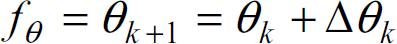
and the system function f(·) as[fx fy fθ]
T
. EKF is implemented as follow: The time update equations (15) and (16) are given by:


where Ak and Bk are the Jacobian matrix of the system and input matrix respectively are obtained by linearization as shown in equation (17) and (18) (Evgeni Kiriy & Martin Buehler, 2002).


For the measurement update, the Jacobian of the function h(·) = [xk yk θk]
T
, measurement matrix Hk is represented in equation (19) as:

The measurement update equations are given by (Evgeni Kiriy & Martin Buehler, 2002):


With these set of equations all the necessary components of EKF have been defined.
The objective to use the Fuzzy Logic Control is to generate the velocities for both the left and the right motors of the robot, which allows the robot to move from start position to goal position. The specification of the control input and output variables have been set. These inputs are: angle θerror which is the difference between the goal angle θg and the current heading θr of robot, the distance derror which is the difference between the current position and the goal position. The calculation is a simple computation of the basic equation between two points. The outputs of Fuzzy Logic Controller are velocities of the left and right motors of the mobile robot. Fig. 8 shows the proposed Fuzzy Logic Controller block diagram.

Schematic diagram for the proposed fuzzy logic controller
Fuzzy logic technique has been used to generate the velocities for each motor of the two wheel mobile robot. The fuzzy logic algorithm is as follows:
Define the linguistic variable(s) for input and output system
Compute two input variables: angle error (the different angle between goal angle and robot's heading) and distance error (the difference between the current position and goal position). Compute two output variables: the velocities of the left and right motors. The fuzzy set values of the fuzzy variables are divided as shown in the Table 2.
Notations for the Fuzzy Logic

The fuzzy set values are set of overlapping values represented by triangular shape that is called the fuzzy membership function. Typical representations of the fuzzy membership function are shown in Fig. 9, Fig. 10 and Fig. 11 below.
Representation of the fuzzy membership functions of angle error Representation of the fuzzy membership functions of velocity output Representation of the fuzzy membership functions of distance error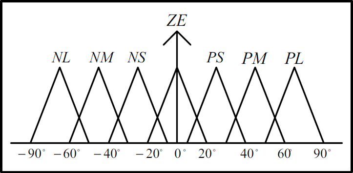


The operation of the system utilizes the fuzzy rules. The notation for making fuzzy logic rules is: Fast Forward (FSFW), Forward (FW), Slow Forward (SLFW), Stop (S), Slow Backward (SLBW), Backward (BW) and Fast Backward (FSBW). The fuzzy rules are shown in the Table 3. and 4. below
Fuzzy rule of the right motor
A typical fuzzy rule of the left motor

Examples of fuzzy rule employed by the path following behavior are shown below:
ℜ1 : ℜ2 :
Defuzzification
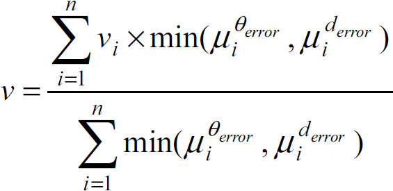
The output action given by the input conditions, the defuzzification computes the velocity output of the fuzzy controller. Centroid defuzzification or Center of Area method calculated by equation (23) as:
where v is defined the fuzzy output of ith rule, μθi error and μiderror are the membership value of the input fuzzy set
Detecting an obstacle
In this research, stereo vision technique has been used for obstacle detection. The flowchart for stereo vision algorithm is shown in Fig. 12. We capture the left and right images at the same time using stereo vision camera. For noise reduction, we used low-pass filter for reducing the noise in the images. Edge detection technique is then used to find edges of each images. In the next step, we find the matched corresponding points between the left and right images. Triangulation method is then applied to calculate the depth for the matched corresponding point. Various tests have been done using the above stereo vision system, We found that an accurate range for obstacle detection is between 0.5 to 6.0 meters.

Typical flowchart of a stereo vision system
The algorithm for obstacle detection is as follows:
If dobs ≥ 0.5 and dobs ≤ 6.0 then
found obstacle(s)
return (xobs, yobs, zobs)
else
not found obstacle(s)
return (0,0,0)
end
where dobs is the distance between the robot and the obstacle.
To avoid the existing obstacles, a series of movement commands must be generated to allow the mobile robot to move pass the obstacles. In order to do so, the program within the mobile robot must analyze the incoming coordinates from 4.4.1. Additional data such as the obstacle angle θobs is calculated which eventually lead to the calculation avoidance angle θavoid for the mobile robot to move through the detected obstacles.

Schematic for obstacle avoidance
The angle θd is the difference between the heading angle θr and the obstacle angle θobs. It's calculated by equation (24) as follow:
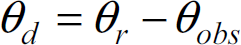
Avoiding angle, θavoid is then calculated as:
if θd < 0 then
θavoid = θg – θobs
else
θavoid = θg + θobs
end
The equations for inputs to the Fuzzy Logic control are as follow:


where θerror is error angle for input fuzzy logic, derror is error distance for inputs to fuzzy logic, θobs is an obstacle angle, θavoid is avoiding angle, θg is goal angle, θr is the heading of the mobile robot, (xg, yg) is a destination position, and (xr, yr) is a current position of the robot.
To improve the precision in the motion control of the robot motion, Extended Kalman Filter, the Fuzzy Logic control and the obstacle avoidance techniques have been implemented. We present the results from the experiments in section 6 to validate the above algorithms.
To test the proposed algorithms, a mobile robot which corresponds to the schematic design has been constructed and is shown in Fig. 4 and Fig 14a. The maximum speed of the robot is approximately 0.45 meters per second. The interfacing circuit of the velocity controller which receives signals from the wheel encoder is shown in Fig. 14a. The interfacing circuit in Fig. 14b also receives signals from the vector compass and the position sensor. In both cases, the DALLAS 89C420 microcontroller has been used. The software interface for the DALLAS 89C420 microcontrollers and sensor module has written in assembly language (MCS-51 family instruction). Software interface for the stereo camera module is written in Microsoft Visual C++ (using vision library from the Point Grey Company). The simulation program is written using MATLAB.

An experimental mobile robot

Interface circuit for the mobile robot controller
The mobile robot with the proposed algorithm has been tested in various unknown environments with obstacles. In all experiments, the robot moved from the start positions to the goal positions correctly and the rest of this section provides results form the simulation experirments performed using the above control algrothm
Simulation Results
The simulations were performed using different maps consisting goal and obstacles.
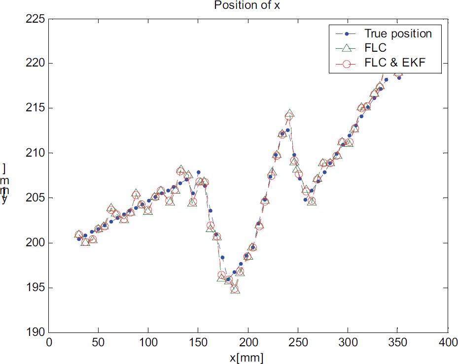
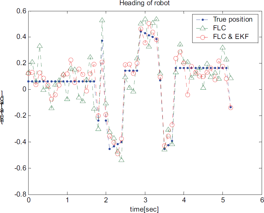
Fig. 15a to show the trajectory followed by the robot avoiding an obstacle on the left hand side of the robot. The simulation results are shown in Fig. 15b, Fig. 15c and Fig. 15d respectively. The “–•–” represents the true position/orientation of the robot motion, the “–Δ–” represents trajectory after the position/orientation error are compensated using the fuzzy logic technique and the “–o–” represents the trajectory after position/orientation errors are compensated by the Kalman Filter and Fuzzy Logic techniques. Fig. 16 and Fig. 17 show similar experiments using other maps. Second simulation experiment (Fig. 16a) has three obstacles in the workspace. The robot moves from start position (30,200) to destination position (350,220). The results changes of xy-position, y-position and heading of robot are show in Fig. 16b, Fig. 16c and Fig. 16d respectively.

The trajectory of the robot movement
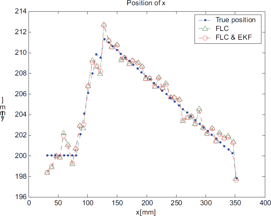
The comparison of robot motion in xy-axis using only FLC and FLC & EKF

The comparison of robot motion in y-axis using FLC and FLC & EKF

The comparison of robot heading using FLC and FLC & EKF

The trajectory of the robot movement
The comparison of robot motion in xy-axis using only FLC and FLC & EKF

The comparison of robot motion in y-axis using FLC and FLC & EKF
The comparison of robot heading using FLC and FLC & EKF
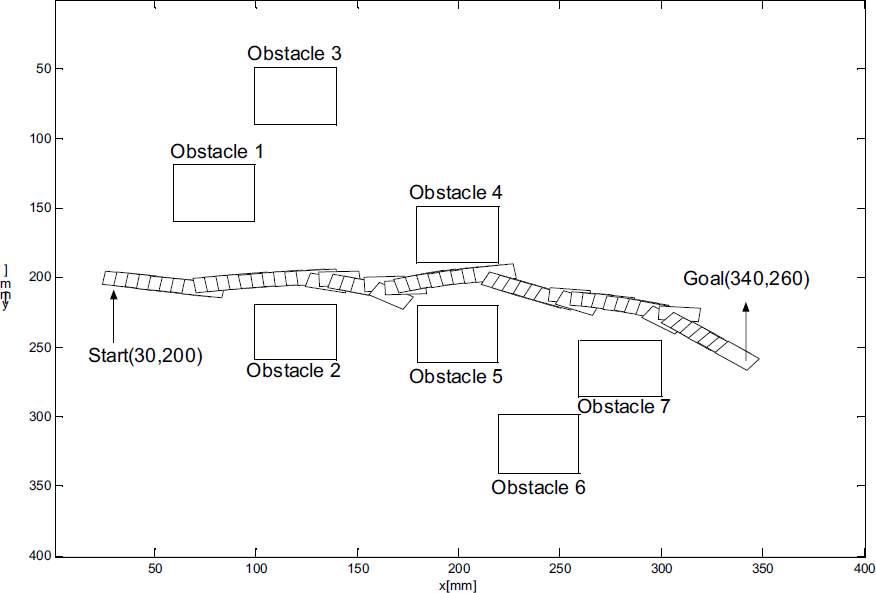
The trajectory of the robot movement
Third simulation experiment, the robot moves from the start position (30,200) to destination position (350,260) by the workspace has seven obstacles (Fig. 17a). Fig. 17b, Fig. 17c and Fig. 17d show the results of xy-position, y-position and heading changes of robot respectively.
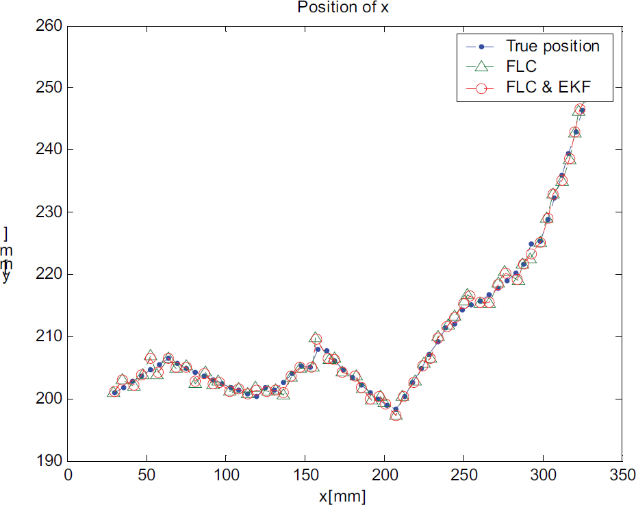
The comparison of robot motion in xy-axis using only FLC and FLC & EKF
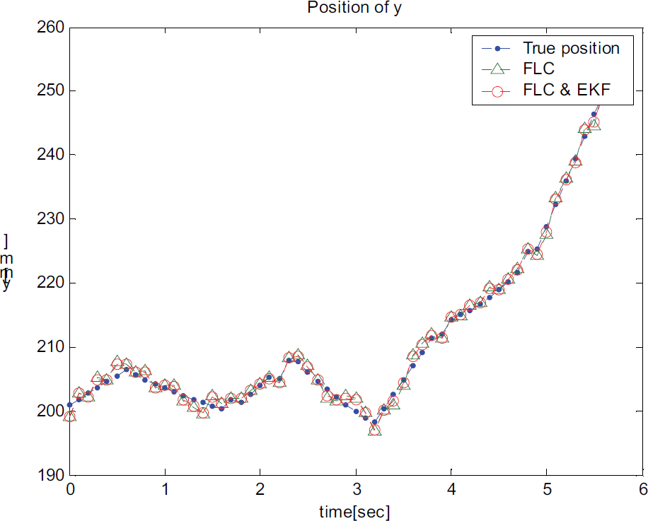
The comparison of robot motion in y-axis using FLC and FLC & EKF
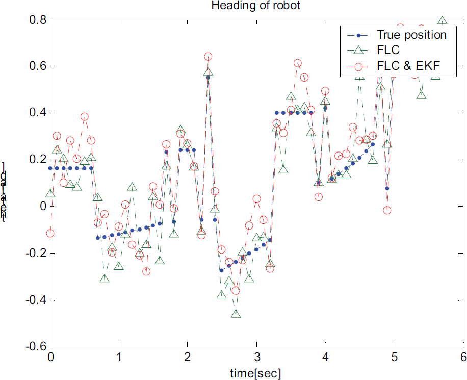
The comparison of robot heading using FLC and FLC & EKF
The quantitative results of the simulation experiments are shown n the above Table 5. From the table we can conclude that, the robot can move from start position to goal position with higher accuracy when FLC and EKF is used together improving the performance of robot motion.
The sample results from the simulation experiments

In this section, the results from two experiments performed in unknown environments such as a corridor (Fig. 18) and a non-linear type passage way (Fig. 19) are presented. Fig. 18 shows a series of snap-shots of the mobile robot passing through an unknown corridor, starts from (a), then proceeds through (b), (c), (d), (e) and finishes at (f).

A typical robot motion passing through an unknown corridor

A typical of robot motion passing through an unknown non-linear type passage way
Similarly in Fig. 19, another series of snap-shot motions passing through an unknown non-linear passage way is shown the robot starts from (a) then passes through (b), (c), (d), (e), (f), (g), (h) and finishes. The ‘Rerngwut I’ robot which has a maximum speed of 0.45 meters per second can move from the starting position, avoid the obstacle, pass through the corridor and reach the goal position successfully in both cases.
This research presents a combination of the Extended Kalman Filter, the Fuzzy Logic Control and the Obstacle avoidance technique which fuses information from different sensors. The proposed system consists of three parts and each of them has it's own function, the Fuzzy Logic technique for the position control, the Extended Kalman Filter technique is for the position predition and correction and the stereo vision technique for the obstacle avoidance. The stereo vision sensor supplies the obstacle detection. The simulations and experiments of robot motion show the results for robot's in which the robot can move from start position to goal position avoiding obstacles in an unknown environment. The proposed algorithm improves the accuracies of the position and the orientation of the robot motion problem. In future work, we propose to apply this algorithm to other platform such as “omni-direction mobile robot” (non-steering wheel type) because it may improve the position and orientation control for achieving a smooth robot motion.