Sage Journals: Discover world-class research

Abstract

This work addresses the problem of metrics for multi-robot systems. It is often desirable to compare different strategies or algorithms for similar problems, e.g. mapping or localization. Since these are often real time applications, classical criterions like time or space complexity are not very helpful. Several other metrics have been suggested. In this paperformation navigation is used as an example application. Possible metrics are presented and discussed, and two of them are used to exemplarily evaluate the results of several formation experiments. Problems and drawbacks of these metrics are discussed and preconditions for a general metricfor the formation problem are adumbrated. Finally, first steps towards a generic and generally applicable metric are presented by means of simulation experiments.

Keywords

Metrics multi robot formation navigation

1. Introduction and Related Work

Research in the field of single robot systems has reached a point where useable solutions have become available. Mathematically well-defined and experimentally proven solutions can be found for the problems of mapping (Thrun et al., 2000), exploration (Burgard et al., 2002), (Burgard et al., 2005), and localisation (Fox et al., 2000). Because quite a lot of experiments have been carried out, in these fields well-elaborated metrics for exact and detailed comparison exist. The situation in the field of multi-robot systems (MRS) is, however, somewhat differ-ent. Various reasons for this include:

The complexity increases with the number of robots.

Most of the single robot methods can not simply be scaled to MRS.

Access to larger real world MRS or adequate Simulation is difficult.

These circumstances might explain the fact that only a few papers deal with systematic (real world) experiments in that field. Additionally, in order to compare algorithms and methods it is important to have measures that allow a meaningful evaluation of the experimental data. One of the popular and also experimental challenging fields in MRS research is formation navigation. By reviewing the literature one will find only sparse and ad-hoc discussions of metrics in this field. The following paper will focus on the problem of developing appropriate metrics for formation navigation.

2. Metrics for Formation Navigation

It is important to have a measure on how well a devel-oped algorithm or method performs. In the area of MRS formation navigation, only a few approaches to expedient metrics can be found.

2.1. Primary Remarks about Metrics for MRS

Metrics are to some extent determined by the scenario in which the MRS operates. Choosing the right parameters requires analysing the experimental set-up carefully. For the rest of the discussion we assume that:

the group of robots is made up of similar types of robots (e.g. all B21 or all Pioneers),

the robots have the ability to communicate with each other,

the robots have the ability to sense the environment and maybe each other (e.g. through track-

real robots operate in a real environment (indoor or outdoor).

Most criteria are very much related to the environment. It has a great influence if the robots operate on an empty soccer field or in a crowded train station. However, most metrics work when measuring the effect of a modification (e.g. new algorithm or parameter set) in exactly the same experimental set-up and infrastructure (same robots, environment etc.).

Reasonable parameters for metrics are:

time

time for travelling

time in / out-of formation

time for setting up / establishing the formation

path

overall path length

path length being in/out-of formation

path length for establishing the formation

position error

displacement in distance

displacement in angle

only for neighbours or for the whole formation

others

Other parameters could be the amount of compu-tation, communication, and sensing.

Looking at the majority of papers in the area of formation navigation, it is obvious that repeatability and reproduci-bility in the sense of a comparison is very difficult. Every real world setup is different even if it is “a typical office environment”. If scientist Calvin would like to compare his approach to scientist Hobbes, he will not be able to do so as long as he has a different setup - at least not if no Transmogrifier is at hand.

One solution for the metric problem might be to take the influence of the environment and other parameters into account. This, of course, would imply that a detailed map of the environment is available, as well as additional information about dynamic objects. This is difficult to achieve in unknown real world scenarios.

2.2. Common Metrics

(Balch and Arkin, 1998) use three performance metrics for evaluation of their formation experiments:

Path length ratio: Path length ratio is the average distance travelled by the robots divided by the straight-line distance of the course.

Average position error: Position error is the average displacement from the correct formation position throughout the run.

Percentage of time out of formation: Percentage of time out of formation reflects the time in which the robots fall out of their formation positions.

(Naffin and Sukhatme, 2004) use similar criteria:

Positional Error: Given a formation, defined as the tuple <G, h, d<, where G is a connected geometric shape, h a desired heading, and d a desired inter-robot spacing, there exist K positions relative to the leader that represent the perfect formation. Given N robots attempting to construct this given formation, where N≤K, they define the formation's positional error as

p = \frac{1}{N} \sum_{i = 1}^{N} D (p_{i}, k_{i}),

where p_i is the i^th robot's position, ki its attempted formation position (both relative to the leader), and D(p_i; k_i) is the Euclidean distance between these two positions. A given set of robots is “in formation” if P < ε, with a user-specified tolerance ε.

Time to convergence: The time to convergence Tc(N) is defined as the duration of time required for a formation to reach a given size N and be in formation for that size.

Percentage of time in Formation: The percentage of time in formation is defined as

F = \frac{t_{i n}}{} where

t_in is the time in formation and t_total is the total time elapsed since the formation reached its current size.

(Fredslund and Matarić, 2002) and (Lemay et al., 2004) use only the formation evaluation criterion Percentage of time in Formation. The robots are considered to be in formation when the following holds:

Given the positions of N mobile robots, an inter-robot distance d_desired, a desired heading h, and a connected geometric shape G (completely characteriseable by a finite set of line segments and the angles between them), then the robots are considered to be in formation G if:

Uniform dispersion: The same distance is kept between all neighbouring robots with a maximum tolerance of $ε_{d_{1}}$ .

$\exists d$ , such that ∀ pairs of immediate neighbours $(R_{i_{1}}, R_{i_{2}})$ with distance dist $(R_{i_{1}}, R_{i_{2}})$ ,

| d - d i s t (R_{i_{1}}, R_{i_{2}}) | < ε_{d_{1}} and | d - d_{d e s t r e d} | < ε_{d_{1}} .

Shape: The robots are at the assigned positions depending on the desired formation with a maximal tolerance of $ε_{d_{2}}$ around the desired position.

No angle in the original shape must be stretched more than ε _a to make the data points fit.

$\exists a$ “stretching function” f with $f (G) = \tilde{G}$ , such that ∀ angles

θ \in G, | f (θ) - θ | < ε_{a},

, and such that ∀ robots R_i, with distance

\begin{matrix} d i s t (R_{i}, \tilde{G}) to \tilde{G}, \\ d i s t (R_{i}, \tilde{G}) < ε_{d_{2}} \end{matrix}

Orientation: The stretching criterion 2 (shape) must not skew the heading more then ε _a .

| f (h) - h | < ε_{a}; for small ε_{d_{1}}, ε_{d_{2}}, ε_{a} > 0

The three criteria allow measuring a “global” position error. Criteria 1 and 2 define tolerances for distance and angle measurements to be able to cope with noise and imprecision. Criterion 3 states that it should be possible to adjust desired distances and angles over the predetermined position so that all robots form the desired shape. The robots are allowed to move in a radius of $ε_{d_{2}}$ away from their desired positions. This criterion enables the realisation of the desired shape even when each robot separately respects criteria 1 and 2.

2.3. Discussion of Metrics

When looking at the three presented approaches, basi-cally, they all use more or less the same metrics:

Position error

Percentage of time in formation

Every time and path parameter that is related to the shape of the formation, can only be calculated when a position error is measured. This reduces the number of elementary metrics for formation navigation to the position error criteria. As already stated above, these parame-ters are highly influenced by the structure of the environment. So, although Balch, Naffin and Fredslund used the same metric, the results cannot be directly compared. To overcome these weaknesses, the influence of the environment must be taken into account. In the normal case of an a priori unknown environment, one approach could be to use the sensor readings coming from obstacles as an influencing factor. By applying a weighting factor, which is inverse proportional to the “density” of obstacles, to the Average Position Error (APE) the influence of the environment can be taken into account. In our approach we use the repulsive obstacle force F_rep to compute this weighting factor (see section 3 for a description). If there are many obstacles the APE must be scaled down to be comparable to an empty environment where F_rep is small.

However, this extension to the formation position error metric is subject to our ongoing work and, therefore, only preliminary results can be shown in section 6. The most part of the experimental evaluation and discussion presented in the following sections addresses only metrics, which do not consider any parameters of the environment. But this is, of course, a necessary step to motivate the need for an extended, generally applicable metric.

3. Our Formation Approach

Before describing the metrics we applied, first a compact description of our formation approach is given. We use a potential field approach as described in (Koren and Borenstein, 1991) and, therefore, assign each robot a specific position inside the target formation. The concept of using a potential field method for controlling a formation is based on the view that not only obstacles and goals can exert forces onto a robot (Borenstein and Koren, 1990). The basic idea is that each robot in a formation can exert repulsive and attractive forces to other robots. These vir tual forces can be used to keep the robots in the desired formation.

As an extension to the similar method presented in (Yamaguchi and Arai, 1994) not only shape-forming forces are used to generate the formation, but also additional types of forces are modelled to achieve a greater flexibility. Two additional forces have to be considered while the formation is forming up or is in motion: the repulsive obstacle forces and the forces, which move the robots towards a certain goal point.

In order to define the virtual formation forces, let $p_{i} \in ℜ^{2}, i = 1, \dots, n$ be the positions of n robots in the formation in an arbitrary Cartesian coordinate system T_F. And let $x_{i} \in ℜ^{2}, i = 1, \dots, n$ be the actual positions of the obots in some world coordinate system T_W. Since we use a so-called directed potential field approach, not only distance information - as in the cited “classical” methods - is used. Additionally, directional information influence the formation forces: Independent of the configuration of T_F in the world coordinate system T_W each robot k expects any other robot at a certain position seen from his own “point of view”. Assuming that robot j already has reached its desired goal position, the expected goal position ${\hat{p}}_{j, k}$ of robot k seen from robot j is

{\hat{p}}_{j, k} = x_{j} + (\begin{matrix} \cos (ω) & - \sin (ω) \\ \sin (ω) & \cos (ω) \end{matrix}) (p_{k} - p_{j}) .

(1)

Thereby, the angle ω is defined as

ω = ϕ_{a c t u a l, k} - ϕ_{g o a l, k^{'}}

(2)

Where

ϕ_{a c t u a l, k} \in [0; 2 π)

is the actual orientation of robot k. If we let

U_{f o r m, j}^{k} (x) = \frac{1}{2} ξ {∥ x - {\hat{p}}_{j, k} ∥}^{2},

(3)

with

U_{f o r m, j}^{k} : R^{2} \to R, j = 1, \dots, k - 1, k + 1, \dots, n

, and ξ a constant scaling factor, then we can define the formation potential

U_{f o r m}^{k} : R^{2} \to R

for each robot k as

U_{f o r m}^{k} (x) = \sum_{\begin{matrix} j = 1 \\ j \neq k \end{matrix}}^{n} U_{f o r m, j} (x) .

(4)

Accordingly, the force $F_{f o r m}^{k} : ℜ^{2} \to ℜ^{2}$ , that applies to a robot k as position x is

F_{f o r m}^{k} (x) = - \nabla U_{f o r m}^{k} (x),

(5)

which can be calculated as follows:

\begin{aligned} F_{f o r m}^{k} (x, y) = & {(\begin{matrix} - \frac{\partial}{\partial x} \sum_{\begin{matrix} j = 1 \\ j \neq k \end{matrix}}^{n} U_{f o r m, j}^{k} (x, y) \\ - \frac{\partial}{\partial y} \sum_{\begin{matrix} j = 1 \\ j \neq k \end{matrix}}^{n} U_{f o r m, j}^{k} (x, y) \end{matrix})}^{T} \\ = & {(\begin{matrix} - \sum_{\begin{matrix} j = 1 \\ j \neq k \end{matrix}}^{n} \frac{\partial}{\partial x} \frac{1}{2} ξ [{(x - {\hat{x}}_{j, k})}^{2} + {(y - {\hat{y}}_{j, k})}^{2}] \\ - \sum_{\begin{matrix} j = 1 \\ j \neq k \end{matrix}}^{n} \frac{\partial}{\partial y} \frac{1}{2} ξ [{(x - {\hat{x}}_{j, k})}^{2} + {(y - {\hat{y}}_{j, k})}^{2}] \end{matrix})}^{T} \end{aligned}

That finally leads to

F_{f o r m}^{k} (x, y) = ξ (\sum_{\begin{matrix} j = 1 \\ j \neq k \end{matrix}}^{n} ({\hat{x}}_{j, k} - x) \sum_{\begin{matrix} j = 1 \\ j \neq k \end{matrix}}^{n} ({\hat{y}}_{j, k} - y)),

(6)

Where $({\hat{x}}_{j, k}, {\hat{y}}_{j, k}) := {\hat{p}}_{j, k} \in R^{2}$ as defined in (1).

Simply worded, for every robot the attractive or repulsive force to (re-) establish the desired formation is calculated with respect to the positions and the orientations of the other robots.

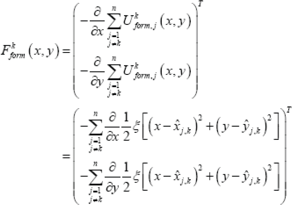
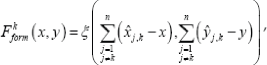
The detailed mathematical definition of obstacle force F_rep and goal force F_att can be found in (Schneider and Wildermuth, 2005). However, in the current implementation we use a simplified approach for the calculation of F_rep The sensor readings are directly transformed into the corresponding repulsive forces. These forces are scaled depending on their distances and, finally, add up. This is of course not mathematically correct, but is fast to compute gives a useable approximation. Altogether, the overall resulting force, which affects a robot k at position x, is

F_{k} (x) = F_{f o r m}^{k} (x) + F_{r e p} (x) + F_{a t t} (x) .

(7)

It is important to re-emphasize that this algorithm differs from the standard potential field approach mainly in the way formation forces are defined. Not only distances are used to define these forces, but also the required angles between the robots and, finally, the direction of the goal as seen from the actual robot positions. Again, see (Schneider and Wildermuth, 2005) for a detailed description and comparison to the standard, non-directed potential field approach to formation navigation.

4. Metrics for the Formation Approach

Based on the formation approach described in the last section we wanted to choose some typical metrics, which one can find in a majority of the cited work. In many cases, special characteristics of a formation algorithm are used to define a metric. Since our goal is a discussion of portability of metrics for different formation approaches, robot systems, and environmental conditions, we tried to avoid this. The two metrics we used for the forthcoming experiments are formation position error and the percent-age of time, for which the robots are “in formation”. As stated in section 2.3 these metrics are also the basic ones used in the described approaches of Balch, Naffin and Fredslund.

In order to compute the formation position error, first an optimal formation position given the actual positions of the robots is calculated. Because of our directed potential field approach, the actual goal point determines the overall direction of the formation. For example, if the target formation is a triangle with one robot in the front, then the triangle formation always is turned with the leader's vertex pointing towards the goal.

This special feature of our formation algorithm simplifies the search for an optimal formation position with regard to the robots' actual positions at each time step. Since the formation direction only depends on the goal and the formation position, for the optimisation only the two-dimensional position parameters have to be considered. Therefore, the function of the added distances between each robot's actual position and its formation position is continuous and monotonically increasing. Thus, a simplex algorithm (Lagarias et al., 1998) with guaranteed termination was used to actually compute the minima. The resulting (minimal) formation position error was used as input for the second metric, the so-called in-for-mation ratio. We chose a threshold of 20cm per involved robot (leading to a 40cm threshold for two robot formations and 60cm for three robots) to decide whether the robots were considered in or out of formation. Of course, these values are somewhat arbitrary, but produced feasible results for our environment (see section 6). A more sophisticated solution should calculate these thresholds automatically in order to keep the presented metrics generic. Influencing factors are, for example, size of robots and environment or density of obstacles (which is often unknown a priori). We are currently evaluating several approaches.

5. Experiments

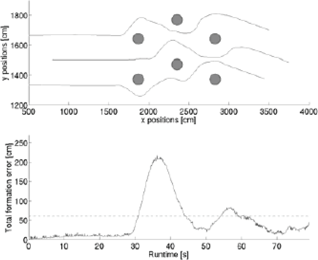
To evaluate the chosen metrics we conducted several experiments, in simulation as well as in our robot lab. In both cases, two identical scenarios have been used. First, the robot formation had to pass a narrow passage of about 3m width and 4m length. In the second scenario, the robots had to move through some regularly positioned pillars. The distance between two pillars of one row was about 3m and the distance between two rows was 2.50m. Fig. 1 gives a graphical illustration of these two settings. For each figure, one simulated example run has been plotted. A formation of two or three robots started on the left side and passed the obstacles, thereby moving towards the goal point on the very right side. The robots used to carry out the experimental runs were all circular with a diameter of 54cm, one iRobot B21 and two Magellans. To get a better impression of our real world set-up look at the pictures in Fig. 2. For the simulated runs, we also modelled round robots of 54cm in diameter. The motion model used in our multi robot simulation environment corresponds to the B21 robot type (Schneider and Wildermuth, 1997).

Fig. 1.

Left: the passage scenario with an exemplarily chosen run of a two robot line formation. Right: The pillar scenario with a three robot triangle formation. The formations started left and moved to the right towards the goal point.

Fig. 2.

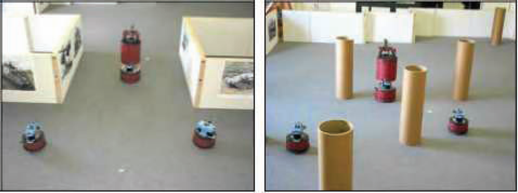
The passage (left) and the pillar scenario (right) in our lab environment. A triangle formation has to pass the obstacles.

In order to apply any metric it is, of course, necessary to acquire precise position information for each robot. Whereas it is simple to get the exact positions from the simulator at a fixed rate of e.g. 10Hz, it is difficult to find this ground truth for any real robot system. Common methods include vision-based approaches using ceiling cameras or specially installed beacons in the environment. Since all our robots are equipped with two SICK laser scanners providing high precision 360 degree distance information, we decided to use a standard SLAM method to correct odometry error and compute global position information for the robots (Dissanayake et al., 2000). The localization step of the chosen SLAM algorithm runs at a much lower frequency than 10Hz and produces correction data only every two to four seconds. Therefore, sometimes gaps occur within the recorded paths of the real robots, because even in a four second interval an additional odometry error of several centimetres can arise. The impact of these inaccuracies is discussed in more detail in section 6.

For both settings, passage and pillars, two different formations have been surveyed, a triangle formation made of three robots and a simple line formation of only two robots. Fig. 1 provides two examples with these two formations. For each combination of two formations and scenarios, 10 runs have been recorded, leading to 40 simulated and 40 real world runs. This data is taken as a basis for the ongoing discussion of the metrics chosen for this multi robot application.

We would like to emphasize that our real world experiments took place in a large experimental area with a size of about 14m × 17m. The set-up included an office like configuration of nearly real world dimensions. This makes the comparison between typical multi-robot experiments (like those carried out by Lemay, Naffin and Fredslund within their work) and our experiments somewhat unbalanced.

6. Results and Discussion

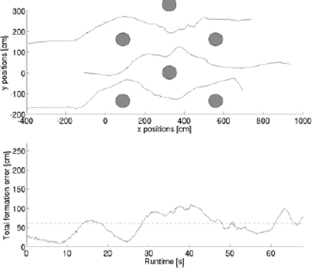
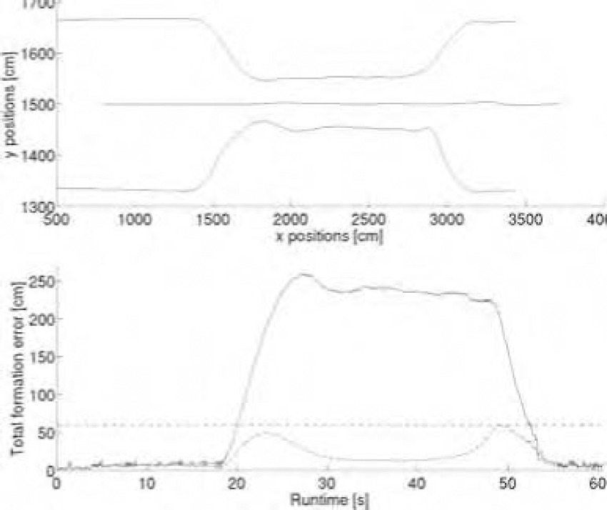
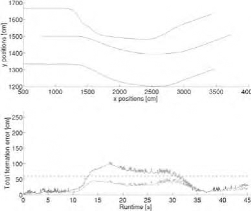
Fig. 3 and Fig. 4 provide two exemplary results for the passage scenario and the two-robot formation shown in Fig. 1 in the last section. Both figures are divided into an upper part, which displays the paths in Cartesian coordinates for both robots, and a lower part, which gives the results in terms of the chosen metrics. The solid line gives the total formation error for each time step, as described in section 3. Additionally, a dashed line is printed showing the limit beyond which the robots are considered to be out of formation. Note that this limit depends on the number of robots, for the two robot case it is 40cm and for three robots 60cm.

Fig. 3.

Results for a two robot formation (two Magellan Pro) passing a small passage. In the following figures, the upper part gives the robot positions (obstacles are added for clarity). The lower part shows the formation error.

Fig. 4.

Simulation results for one example run with two robots in the passage scenario.

Fig. 3 presents data recorded with real robots in our multi robot lab, Fig. 4 refers to an arbitrarily chosen simulation run. As one can see, results are similar concerning both the maximum formation error as well as the information ratio. Before a deeper discussion of the numerical results, examples for the other treated scenario are given.

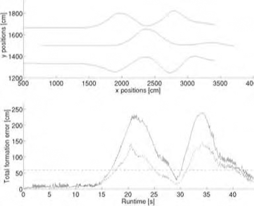
Fig. 5 and Fig. 6 picture the data generated during two example runs of three robots in a triangle formation passing the pillar scenario. In contrast to the results from the passage, now there are major differences between real robots and simulation. Looking at the formation error chart, one can find that the mean error is smaller for the simulation run. On the one hand, this is because the simulated robots always move somewhat “smoother”, especially near obstacles, which leads to slightly larger position errors for the real robots. On the other hand, as already stated in the last section, it is difficult to localize the robot positions exactly, even in a lab environment. This additional error is hard to quantify, in terms of size as well as in terms of distribution. For a compensation of this error, a very precise localisation or additional information about the nature of the robots' odometry error is needed. Since both is hard to achieve in real world envi-ronments, we simply treat the robot positions as “precise”. Any refinement is subject to future work. Although the mean error is smaller in simulation, the maximum of about 220cm is almost twice as large as in the lab run with real robots. The reason for this is obvious when looking at Fig. 7 and Fig. 8: these charts compare the robots' actual paths (solid line) and the computed optimal formation paths (dotted lines with different markers). See section 4 on how this calculation is done. The robot, which starts at the lower left position, in simulation passes the first obstacle “on the wrong side”, leading to a temporarily very large formation error. How-ever, this type of wrong path decision occasionally hap-pens for both the real lab runs as well as the simulation runs. Therefore, the mean of the 10 recorded runs is influenced in the same way for lab and simulation experi-ments.

Fig. 5.

Three robots (one B21 and two Magellan Pro) in a triangle formation, pillar scenario.

Fig. 6.

Example run for three simulated robots in triangle formation in the pillar scenario.

Fig. 7.

Deviance between the paths of the 3 robots in the triangle formation (solid lines) and their optimal formation positions (dotted lines).

Fig. 8.

Deviance between the paths of the 3 robots in the triangle formation (solid lines) and their optimal formation positions (dotted lines), simulation runs.

Table 1 and Table 2 provide some numerical results, namely the mean and the standard deviation for the two chosen metrics. Table 1 gives the results for the different scenarios and the different formations (two robots in a line, three in a triangle) for real laboratory runs, whereas Table 2 lists these values for the simulation runs. What can be seen corresponds well to the results stated so far. The formation error for the passage scenario is much larger than for the pillars, which is, of course, because, while moving through the passage, two robots are far out of formation. Nevertheless, the results for real world and simulation are similar. On the other hand, for the pillar scenario simulation results are better, for the reasons mentioned before. Nevertheless, because of the occasional large errors in this scenario (due to “wrong ways”, see Fig. 8) the standard deviation is very large. The information ratio metric gives similar results. For the pillar scenario, the ratio is better, but at the same time, the standard deviation is much larger. It is worth mentioning, that the range of the resulting values is quite low. In most of the runs, the robots were out of formation for more than half of the time. This, of course, leads to the question whether this is a suitable metric for obstacle scenarios.

Table 1.

Numerical results for lab runs: total formation error and information ratio, 10 runs each, with standard deviation.

	Formation error (cm)	Std. dev.	Formation ratio	Std. dev.
Passage 2 robots	87.1357	2.3418	0.4527	0.0319
Passage 3 robots	116.0297	6.9447	0.3770	0.0325
Pillars 2 robots	49.0801	15.9714	0.5675	0.1477
Pillars 3 robots	71.5922	29.3875	0.4838	0.2271

Table 2.

Numerical results for simulation, also 10 runs each, with standard deviation.

	Formation error (cm)	Std. dev.	Formation ratio	Std. dev.
Passage 2 robots	93.1811	0.4685	0.4974	0.0025
Passage 3 robots	121.7899	10.1445	0.4783	0.0085
Pillars 2 robots	38.8999	21.4419	0.6982	0.1787
Pillars 3 robots	56.0451	17.3125	0.7171	0.0786

Note, however, that all mentioned differences in the results are solely caused by special characteristics of the environment. On the one hand, there is the rather small impact of simulated or real world runs. Nevertheless, everything else remains the same, including the algorithms, the robots, the simulator, and the laboratory. Just the choice of obstacles leads to the major changes in the results. Thus, it is worth asking what results the same metrics would have produced with another type of robots in another lab environment and other obstacles - and how comparable these results can be.

Fig. 9.

The weighted formation error (dashed line) for the passage scenario and a triangle formation; compare with Fig. 4.

Fig. 10.

A triangle formation passing a wall on their left. Non-weighted (solid line) and weighted (dashed line) formation error.

7. Overview and Ongoing Work

In this paper, the problem of general metrics for multi-robot applications has been addressed. The task of formation navigation was used as base for the discussion. After a short outline of several suggested metrics for this application, two exemplary metrics were applied to simulated and real world formation experiments. Although using the same robots and the same algorithms, the metrics produced very different results - being highly dependent on the structure of environment and obstacles.

Fig. 11.

Non-weighted (solid line) and weighted total formation error (dashed line) for the pillar scenario and a triangle formation.

As mentioned in section 2.3 the next step towards a general metric, i.e. one that is at least independent of the surroundings is to use information about the environment as additional parameter. Some preliminary experiments have been conducted using such information for scaling the formation error for each robot. It is important to mention that we consider the environment to be a priori unknown and possibly non-static. Therefore, only actual sensor information is used for calculations. Fig. 9 shows that with this enhancement the (weighted) formation error metric now correctly reflects the fact that in the passage scenario the formation is only “com-pressed”. The same holds for Fig. 10 that provides a simi-lar example, in which a three-robot triangle formation avoids a wall-like obstacle on their left. In both figures the upper part shows the robots' paths and the lower part compares non-weighted (solid line) and weighted (dashed line) total formation error. In both cases the weighted formation error drops below the information threshold during the whole run, meaning that the three robots are considered to form a still acceptable triangle formation while avoiding the obstacles (see section 4 for a detailed description of the in-formation ratio metric). Fig. 11 gives an example of a triangle formation in the “pillar” scenario. See section 6, especially figures Fig. 6 and Fig. 8, for a detailed description of the environment.

Now the weighted formation error metric correctly reflects the fact, that the formation is really distorted twice while passing the obstacles, meaning that the robots choose the “wrong side” when they pass some of the pillars. Whenever this happens, the total formation error (non-weighted and weighted) grows up to 150cm or above, which is more than twice the in-formation threshold.

Table 3 summarizes the results of these preliminary experiments numerically. For all scenarios – “wall”, “passage”, “pillars”, each with 3 robots in a triangle formation – we recorded 10 simulated runs and computed mean values for the total formation error and the in-formation ratio, as well as their standard deviations. As stated above for the arbitrarily chosen example runs, when looking at the first two scenarios then, according to the weighted metric, the three robots are perfectly in formation throughout all of the “passage” and “wall” runs. For the “pillars” the mean formation error is also much lower using the weighted version of the metric. However, since the robots often leave their positions inside the triangle formation, by means of the in-formation ration they are still considered to be out of formation nearly half of the time.

Table 3.

Comparison between non-weighted and weighted formation metrics for different scenarios. For each scenario 10 simulation runs with three robots in a triangle formation have been evaluated.

	Non-weighted metrics				Weighted metrics
	Formation error (cm)	Std. dev.	Formation ratio	Std. dev.	Formation error (cm)	Std. dev.	Formation ratio	Std. dev.
Wall	42.2076	1.2901	0.6230	0.0431	22.9893	0.9714	1	0
Passage	109.0772	5.5965	0.4759	0.0077	16.4216	0.8488	1	0
Pillars	85.8374	17.4192	0.5087	0.0645	51.0063	10.5177	0.6346	0.0883

Although these results look promising, for a sensible comparison of different approaches, tested with different robots in different laboratories, even more parameters must be taken into account. Nevertheless, it is definitely worth continuing work on extended, generally applicable metrics, since the only other feasible way of measuring quality of results is to enforce identical experimental conditions by designing more and more specialised robot competitions.

References

Balch

, and Arkin

R. C.

(1998). Behaviour-based Formation Control for Multi-robot Teams. IEEE Transactions on Robotics and Automation, Vol. 14, No. 6, pp. 926–939.

Borenstein

, and Koren

, (1990). Real-time Obstacle Avoidance for Fast Mobile Robots in Cluttered Environments. Proc. of 7 IEEE International Conference on Robotics and Automation. Cincinnati, Ohio, pp. 572–577.

Burgard

Moors

, and Schneider

F. E.

(2002). Collaborative Exploration of Unknown Environments with Teams of Mobile Robots. In Beetz

Hertzberg

Ghallab

, and Pollack

M. E.

, editors, Advances in Plan-Based Control of Robotic Agents. Springer Verlag, Vol. 4266 of Lecture Notes in Computer Science.

Burgard

Moors

Stachniss

, and Schneider

F. E.

(2005). Coordinated Multi-Robot Exploration. IEEE Transactions on Robotics, to appear.

Dissanayake

Durrant-Whyte

, and Bailey

(2000). A computationally efficient solution to the simultaneous localization and map building (SLAM) problem. Proc. of the ICRA2000 Workshop on Mobile Robot Navigation and Mapping, San Francisco, USA.

Fox

Burgard

Kruppa

, and Thrun

(2000). A Probabilistic Approach to Collaborative Multi-Robot Localization. Autonomous Robots, 8 (3).

Fredslund

, and Matarić

M. J.

(2002). A General Algorithm for Robot Formations Using Local Sensing and Minimal Communication. In IEEE Transactions on Robotics and Automation, Special Issue on Multi Robot Systems. 18(5):837–846.

Koren

, and Borenstein

, (1991). Potential Field Method and Their Inherent Limitations for Mobile Robot Navigation. Proc. of 8 IEEE International Conference on Robotics and Automation, Sacramento, pp. 1398–1404.

Naffin

, and Sukhatme

(2004). Negotiated Formations. Proc. of the International Conference on Intelligent Autonomous Systems, pp. 181–190.

10.

Lagarias

J. C.

Reeds

J. A.

Wright

M. H.

, and Wright

P. E.

(1998). Convergence Properties of the Nelder-Mead Simplex Method in Low Dimensions. SIAM Journal of Optimization, Vol. 9 No. 1, pp. 112–147.

11.

Lemay

Michaud

Létourneau

, and Valin

J.-M.

(2004). Autonomous Initialization of Robot Formations. Proc. of the IEEE Intern. Conference on Robotics and Automation (ICRA), New Orleans, USA.

12.

Schneider

F. E.

, and Wildermuth

(1997). Simulation von Mehrrobotersystemen. Proc. of the 13th Fach-gespräch Autonome Mobile Systeme (AMS), Stuttgart, Germany.

13.

Schneider

F. E.

, and Wildermuth

(2005). Directed and Non-Directed Potential Field Approaches to Formation Navigation. Proc. of the 2^nd IASTED International Conference on Automation, Control, and Applications (ACIL-ACA 2005), Novosibirsk, Russia.

14.

Thrun

Burgard

, and Fox

(2000). A Real-Time Algorithm for Mobile Robot Mapping with Applications to Multi-Robot and 3D Mapping. Proc. of the IEEE International Conference on Robotics & Automation.

15.

Yamaguchi

, and Arai

, (1994). Distributed and Autonomous Control Method for Generating Shape of Multiple Mobile Robot Group. Proc. of International Conference on Intelligent Robots and Systems, Federal Armed Forces University Munich, pp. 800–807.

Discussion of Exemplary Metrics for Multi-Robot Systems for Formation Navigation

Abstract

Keywords

1. Introduction and Related Work

2. Metrics for Formation Navigation

2.1. Primary Remarks about Metrics for MRS

2.2. Common Metrics

2.3. Discussion of Metrics

3. Our Formation Approach

5. Experiments

References