Sage Journals: Discover world-class research

Abstract

The present work proposes an improved geodesic algorithm for the trajectory planning of multi-joint robots. First, all of the joint variables are chosen to set up a generalized local coordinate system for the product of the positional space and the orientational one. Second, by defining a new Riemannian metric that contains both the positional and rational parameters, the traditional geodesic algorithm is improved so that it becomes capable of planning robot trajectories that include both the position and the orientation. To demonstrate the effectiveness of the improvement, trajectories are planned for two typical joint robots: one being a planar 3R and the other a spatial RRPP. It is verified that the improved algorithm can generate not only smooth motions for the joints but also smooth and accurate motions for the end-effector. The improved algorithm applies to multi-joint robots with no more than six degrees of freedom.

Keywords

trajectory planning multi-joint robot geodesic Riemannian metric smooth motion

Introduction

Trajectory planning is a fundamental problem in the design of multi-joint robots.¹ The polynomial-function-based methods are widely used to plan robot trajectories. Although the linear and parabolic polynomials can meet the requirement of trajectory in some simple cases,² they often lead to discontinuous interpolation, which sometimes gives rise to unsatisfactory planning results. To overcome this shortcoming, higher-order (such as cubic and quartic) polynomials are instead employed to conduct trajectory planning.^1,3,4 In this respect, the most frequently used interpolation functions are splines which are piecewise polynomials, including the cubic splines^5,6 and the B-splines.^7,8

These polynomials-based methods are generally employed to plan the robot trajectories at the joint level, which inevitably leads to inaccurate movements of the end-effector in the Cartesian space. To enhance the motion precision of the end-effector, one method is to convert its Cartesian path into the joint trajectories at some intermediate points (called knots). The trajectory segments between any neighboring knots can then be calculated by interpolation. Although this method guarantees the accuracy of the knot positions in the Cartesian space, the trajectory of the end-effector is unforeseeable, because it involves no forward kinematic calculation.

Besides polynomials, geodesic functions can also be used to plan trajectories for joint robots.^9

–13 The fundamental idea of the geodesic-based trajectory planning method is to replace line or arc segments in a Euclidean space by geodesics in a Riemannian manifold. Because a geodesic curve generally represents (locally) the shortest path between two points in a Riemannian manifold,¹⁴ the geodesic-based method can always yield an optimal trajectory.

Some literature addressed the geodesic trajectory planning in the joint space.^15,16 In order to generate joint trajectory by the geodesic method, inverse kinematic analysis has to be performed.¹⁵ However, it is usually a difficult work to get a constant solution to the inverse kinematic equations. To avoid the troublesome inverse kinematic analysis, Selig and Ovseevitch employed the group theory to describe the geodesic paths in the joint space.¹⁶

In addition to the group theory, the theory of Riemannian geometry can also be directly used to make the geodesic trajectory planning easy to operate.¹⁰ This involves two main steps. First, the Riemannian metric needs to be constructed according to the planning task; second, the trajectories are planned by solving the geodesic equations. Either the distance or the kinetic energy can be chosen as the Riemannian metric to achieve the optimal trajectory with the minimum distance or minimum kinematic energy.¹⁷ Because only the positional parameters are considered, the distance-based Riemannian metric cannot be used to tackle the orientation problems that involve the rotational parameters. Due to this reason, when the distance metric is chosen as the Riemannian metric, the geodesic method is unsuitable to be applied in planning trajectories for both planar 3R robots and multi-joint robots with more than three degrees of freedom (DOFs). In this case, it has been demonstrated that not all of the joint trajectories of the Kuka youBot arm that has five joints can be planned by the geodesic method.¹⁰

By constructing a Riemannian metric that contains both the positional and rotational parameters, the present paper proposes an improved geodesic algorithm for trajectory planning. Because the rotational parameters are included into the Riemannian metric, the improved algorithm can be used to tackle the orientational problems, and thus it can be applied in trajectory planning for both planar 3R robots and multi-joint robots with no more than six DOFs. It is demonstrated by two examples that the improved algorithm can yield not only smooth motions for the joints but also smooth and accurate trajectories for the end-effector.

The improved geodesic trajectory planning algorithm

Geodesics are natural generalization of lines. A geodesic is (locally) the shortest path between points in a Riemannian manifold. Constructing different manifolds and Riemannian metrics, one can obtain different geodesics such as lines, arcs and paths of minimum distance or minimum kinetic energy.

Assume that M is a Riemannian manifold and g is a Riemannian metric of M. In general, the Riemannian metric can be represented as

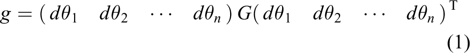
g = (\begin{array}{l} d θ_{1} & d θ_{2} & \dots & d θ_{n} \end{array}) G {(\begin{array}{l} d θ_{1} & d θ_{2} & \dots & d θ_{n} \end{array})}^{T}

where $G = (g_{i j})_{n \times n}$ is the coefficient matrix of the Riemannian metric; $θ_{i}, (i = 1, \dots, n)$ are joint positions which can be linear or angular; and ‘d‘ denotes the differential operator.

It is desirable to deduce equations describing the geodesic paths in the joint space. Let $γ : I \to M$ be a smooth curve, where I is an interval. In a local coordinate system {θ_i} (the definition of local coordinate system will be given later), a curve can be written as

θ_{i} = θ_{i} (s), (s \in I; i = 1, 2, \dots, n)

We say that γ is a geodesic if and only if it satisfies the geodesic equations

\frac{d^{2} θ_{i}}{d s^{2}} + \sum_{k, j = 1}^{n} Γ_{k j}^{i} \frac{d θ_{k}}{d s} \frac{d θ_{j}}{d s} = 0 (i = 1, 2, \dots, n)

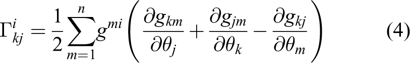
The Christoffel symbols $Γ_{k j}^{i}$ are given in terms of the Riemannian metric by

Γ_{k j}^{i} = \frac{1}{2} \sum_{m = 1}^{n} g^{m i} (\frac{\partial g_{k m}}{\partial θ_{j}} + \frac{\partial g_{j m}}{\partial θ_{k}} - \frac{\partial g_{k j}}{\partial θ_{m}})

where g^mi is the element of G⁻¹.¹⁸

The solution of (3) with boundary conditions gives the joint trajectories. The flow graph of the geodesic algorithm is shown in Figure 1.

Figure 1.

Flowchart of the geodesic algorithm.

The key step is to construct a Riemannian manifold M and its Riemannian metric g such that a geodesic of the Riemannian manifold is the planned path.

We take all of the possible positions and orientations of a robot as a Riemannian manifold M which is the product manifold of the position space and the orientation space. To be specific, M consists of all possible positions and orientations, $\hat{p} = (n, o, a, p)$ , where p is the end-effector position and the rotation matrix R = (noa) represents its orientation.¹ The Riemannian metric is defined by

g = g_{1} + g_{2}

where $g_{1} = (d p)^{2}$ (p is the end-effector position vector) is the distance metric of M₁, and g₂ is a perturbation component to ensure that the metric g is a positive-definite quadratic form. Because a quadratic form can be written as the sum of squares by the applying the non-singular linear transformations,²⁰ it follows that the perturbation component g₂ can also be written as a form of sum of squares. In order to optimize the orientation, we define g₂ as

g_{2} = (d n)^{2} + {(d o)}^{2} + {(d a)}^{2}

Then, the Riemannian metric becomes

g = d {\hat{p}}^{2} = (d p)^{2} + {(d n)}^{2} + {(d o)}^{2} + {(d a)}^{2}

Obviously, the Riemannian metric contains not only the positional parameters but also the rotational ones.

For robots, the kinematical equations give a description from the joint space to the Cartesian space. Because the kinematical equations are nonlinear, the inverse solution is not always unique. There is always no one-to-one mapping between the Cartesian space and the joint space. For this reason, we cannot directly take all the joint variables as the coordinate system of the Cartesian space. In order to solve this problem, local coordinates are introduced.

Assuming U is a neighbourhood of a manifold M. If $ϕ : U \to ϕ (U) \subset R^{n} (ϕ (U)$ is open) is the homeomorphism and denote $θ_{i} (Q) ≐ {(ϕ (Q))}_{i}, (U; θ_{i})$ is a local coordinate system of M and $θ_{i} (i = i, \dots, n)$ are local coordinates.¹⁹

When the joint variables can be regarded as local coordinates of M, for an arbitrary point Q₀ ∈ M and a neighbourhood of Q₀, U, the inverse solutions of Q₀ may be not unique. Without lost of generality, assume there are two inverse solutions $θ_{i}^{(1)}$ and $θ_{i}^{(2)} (i = i, \dots, n)$ . Let V₁ and V₂ denote neighbourhoods of θ⁽¹⁾ and θ⁽²⁾, respectively, which satisfy $x (V_{1}) = U, x (V_{2}) = U$ , where x = x(θ) is the forward kinematics equation. Define $ϕ : U \to V_{1} \subset R^{n}$ as follows

{\begin{cases} ϕ (Q_{0}) & = & θ^{(1)} \\ ϕ (Q) & = & \begin{array}{l} x^{- 1} (Q {) |}_{V_{1}}, & Q \in U \end{array} \end{cases}

Here ϕ is a homeomorphism mapping and $θ_{i} (Q) ≐ {(ϕ (Q))}_{i}$ are local coordinates. The mappings of the local coordinates are shown in Figure 2.

Figure 2.

Mappings of local coordinates.

After the Riemannian metric is constructed, the geodesics on the product space can be obtained by (3). It deserves nothing that the geodesics represented by joint variables are on the product space, but it is desirable to describe the planned trajectory on the positional space with a specific shape such as a line. Therefore, we need to pull the geodesics back to the positional space to obtain an accurate Cartesian path. For a given embedding $φ : M_{1} \to M$ and a geodesic $γ : I \to M$ , the pull-back of γ is defined as follows

φ^{*} γ (s) = φ^{- 1} \circ γ (s), (s \in I),

where φ*γ is the pullback of γ. The diagram of the pull-back is shown in Figure 3. The immediate output of the geodesic algorithm is joint trajectories. The motion performed by the robot end-effector is exactly a geodesic path.

Figure 3.

A diagram of the pull-back.

When g₂ = 0, the improved geodesic algorithm degenerates to the traditional one, i.e. $g = g_{1} = (d p)^{2}$ . Because the Riemannian metric of the traditional geodesic algorithm only contains the positional parameters, the coefficient matrix G will become singular, if there are more than three DOFs. Due to this reason, the traditional geodesic algorithm can only be used to plan trajectories for planar 2R and spatial 3R robots.¹⁰ As shown in (7), the improved Riemannian metric contains not only the positional parameters but also the rotational ones so that the coefficient matrix G will not become singular when the DOFs are more than three. Therefore, the improved geodesic algorithm can be used to plan trajectories for multi-joint robots with more than three DOFs.

In addition, when the metric is defined as (7), the manifold we focus on is position and orientation space which is at most six dimensional. The amount of joints which can be selected as local coordinates $θ_{i} (i = 1, \dots, n)$ is at most six, i.e. n ≤ 6.

The properties of the improved algorithm

Effect of the perturbation component

Let us do a thorough study on the effect of the perturbation component g₂.

Lemma 1. The trajectory planned by the geodesic algorithm is a geodesic.

Proof. For low-DOF robots, if we take the Riemannian metric as $g = g_{1} = (d p)^{2}$ , the trajectory planned by the geodesic algorithm is a geodesic. Because the calculation of a geodesic is on the joint space and the positional space, no pullback is needed. For multi-DOF robots, if (7) is taken as the Riemannian metric, we need to show that the pullback of a geodesic is a geodesic.

Given Riemannian manifolds $(M_{1}, g_{1})$ and $(M_{2}, g_{2}), M_{1} \times M_{2}$ is the Riemannian product of M₁ and M₂. Assume that P and Q are the projection mappings from $T (M_{1} \times M_{2})$ to TM₁ and TM₂, respectively, where TM denotes the tangent space of M. The Riemannian metric of $M_{1} \times M_{2}$ is defined by $g (X, Y) ≐ g_{1} (P X, P Y) + g_{2} (Q X, Q Y)$ . Then, both M₁ and M₂ are all geodesic submanifolds of $M_{1} \times M_{2}$ .²² If M₁ is the positional space and $M = M_{1} \times M_{2}$ is the position and orientation space, M₁ is a geodesic submanifold of M. That is, assuming that $φ : M_{1} \to M$ is an embedding and γ is a geodesic of M, the pullback of γ (i.e. φ*γ) is a geodesic of M₁. □

From Lemma 1, the perturbation component g₂ will not make a perturbation when no simplification is made. It is not easy to find and describe the embedding and the pullback. In Section 4, we will make simplifications and take the projection of a geodesic from M to M₁ as the trajectories of the positional space and the joint space. The perturbation may take place when we replace the geodesic pull-back by the projection. The longer the distance is, the more evident the perturbation will be.

Output controllability

Lemma 2 The velocity of the trajectory planned by the geodesic algorithm is controllable.

Proof. From Section 3.1, the trajectory planned by the improved algorithm is either a geodesic or the projection of a geodesic (a simplified case). First, we declare that the velocity of a geodesic is controllable. If a geodesic $γ (s, v)$ (v is the initial velocity of γ) is defined on $s \in (- ε, ε)$ , then $γ (s, λ v), (λ > 0)$ is also a geodesic that is defined on $s \in (- \frac{ε}{λ}, \frac{ε}{λ})$ ; moreover, $γ (s, λ v) = γ (λ s, v)$ .²¹ This means that the initial velocity can be controlled by adjusting the range of parameter s. Because a geodesic generally has constant speed (the norm of speed is constant),¹⁸ the velocity of a geodesic is controllable. Second, the velocity of the geodesic projection is still controllable. Because the velocity of a geodesic on the position and orientation space is controllable, the velocity of the geodesic projection from the position and orientation space to the position space is also controllable. □

Because of Lemma 2, we can adjust the velocity to make the robot move the entire distance in a given time. Thus, in the following simulations, we simply take a unified convention that the parameter s always ranges from 0 to 1. One can change the interval of the parameter s to meet other demands. If the velocity of a geodesic is set to be 1, the parameter s stands for the arc length. If parameter s is time, the motion time can be predefined. In this way, time optimal trajectory planning can be realized, as the time can be optimized to meet the kinematical constraints.

Trajectory scalings

Problem 1. Given a space M and two points x₀, x₁ ∈ M, with no other constraints, how should we choose our interpolant $x : [0, T] \to M, T > 0$ so that $x (0) = x_{0}, x (T) = x_{1} ?$

Here, we can choose a geodesic to connect the two points. If the given points were specified as $x_{0}, x_{1}, \dots, x_{n}, (n > 1)$ , we might choose x to be a piecewise-geodesic, which is usually not differentiable at the junctions. There is frequently a jump discontinuity of velocity curves at the junctions. With Lemma 2, we can perform trajectory scalings to reduce the gaps. Assume that x₁ is a junction, $γ_{1} (s) (s \in [0, T_{1}])$ is a geodesic connecting x₀ and x₁, and $γ_{2} (t) (t \in [T_{1}, T_{2}])$ is another geodesic connecting x₁ and x₂. Denote ${γ^{'}}_{1} (0) = v_{0}, {γ^{'}}_{2} (T_{1}) = v_{1} (| v_{0} | \neq | v_{1} |)$ . Because a geodesic has constant speed, $| {γ^{'}}_{1} | = | v_{0} |$ and $| {γ^{'}}_{2} | = | v_{1} |$ . We scale γ₂ to reduce the gap between γ₁ and γ₂. As mentioned in Section 3.2, $γ (s, λ v) = γ (λ s, v), λ > 0$ . By means of this property, $γ_{2} (t, v_{2}) = γ_{2} (\frac{1}{λ} t, λ v_{2}) . | v_{0} | = | λ v_{2} |$ requires $λ = \frac{| v_{0} |}{| v_{1} |}$ . Set

γ_{3} (u, v_{2}) = γ_{2} (\frac{| v_{0} |}{| v_{1} |} u, v_{1}), u \in [T_{1}, T_{1} + \frac{| v_{1} |}{| v_{0} |} (T_{2} - T_{1})],

where $v_{2} = \frac{| v_{0} |}{| v_{1} |} v_{1}$ . Then ${γ^{'}}_{3} (T_{1}) = v_{2}$ , and $| {γ^{'}}_{3} | = | {γ^{'}}_{1} | = | v_{0} |$ . So $γ_{3} (u, v_{2}) (u \in [T_{1}, T_{1} + \frac{| v_{1} |}{| v_{0} |} (T_{2} - T_{1})])$ is a scaling of γ₂ which reduces the gap between the velocity curves of γ₁ and γ₂. Here γ₂ should be replaced by γ₃. Because of the definition of γ₃, the paths are the same geodesic when γ₂ and γ₃ are mapped into the Cartesian space.

When the projection of a geodesic is taken as the trajectory and perturbations arise, we can select several points on the shortest path that connects the initial point and the end point. Applying the improved algorithm to each neighbouring pair, we obtain a piecewise-geodesic that is still a line when it is mapped into the positional space. With the trajectory scaling as mentioned above, the piecewise-geodesic can be second-order continuous at the junctions. One can smooth the piecewise-geodesic at the junctions when higher-order continuity is needed.

Simulations

The improved geodesic algorithm for a planar 3R robot

A planar 3R robot is shown in Figure 4, where $l_{i}, θ_{i} (i = 1, 2, 3)$ denote linkage lengths and rotatory angles, respectively. The Riemannian metric is defined as follows

\begin{array}{l} g & = & {(d p)}^{2} + {(d n)}^{2} + {(d o)}^{2} + {(d a)}^{2} \\ = & (\begin{matrix} d θ_{1} & d θ_{2} & d θ_{3} \end{matrix}) G {(\begin{matrix} d θ_{1} & d θ_{2} & d θ_{3} \end{matrix})}^{T} \end{array}

where

{\begin{array}{l} p = & (c_{1} l_{1} + c_{12} l_{2} + c_{123} l_{3}, s_{1} l_{1} + s_{12} l_{2} + s_{123} l_{3},0) \\ n = & (c_{123}, s_{123},0) \\ o = & (- s_{123}, c_{123},0) \\ a = & (0, 0, 1) \end{array}

$G = (g_{i j})_{3 \times 3}$ is the coefficient matrix of the Riemannian metric, and its elements are

{\begin{array}{l} g_{11} & = & 2 + {(s_{23} l_{1} + s_{3} l_{2})}^{2} + {(c_{23} l_{1} + c_{3} l_{2} + l_{3})}^{2}, \\ g_{12} & = & g_{21} = 2 + l_{2}^{2} + 2 c_{3} l_{2} l_{3} + l_{3}^{2} + l_{1} (c_{2} l_{2} + c_{23} l_{3}), \\ g_{13} & = & g_{31} = 2 + l_{3} (c_{23} l_{1} + c_{3} l_{2} + l_{3}), \\ g_{22} & = & 2 + l_{2}^{2} + 2 c_{3} l_{2} l_{3} + l_{3}^{2}, \\ g_{23} & = & g_{32} = 2 + c_{3} l_{2} l_{3} + l_{3}^{2}, \\ g_{33} & = & 2 + l_{3}^{2} \end{array}

Figure 4.

A planar 3R robot.

The corresponding geodesic is determined by (3) and (4). By calculation, we get

{\begin{array}{l} Γ_{11}^{1} & = - \frac{c_{2} l_{1} + l_{2} + c_{3} l_{3}}{s_{2} l_{1}}, Γ_{12}^{1} = Γ_{21}^{1} = Γ_{22}^{1} = - \frac{l_{2} + c_{3} l_{3}}{s_{2} l_{1}}, \\ Γ_{13}^{1} & = Γ_{31}^{1} = Γ_{23}^{1} = Γ_{32}^{1} = Γ_{33}^{1} = - \frac{c_{3} l_{3}}{s_{2} l_{1}}, \\ Γ_{11}^{2} & = \frac{1}{s_{2} l_{1} l_{2}} (l_{1}^{2} + l_{2} (l_{2} + c_{3} l_{3}) + l_{1} (2 c_{2} l_{2} + c_{23} l_{3})), \\ Γ_{12}^{2} & = Γ_{21}^{2} = Γ_{22}^{2} = \frac{l_{2} (l_{2} + c_{3} l_{3}) + l_{1} (c_{2} l_{2} + c_{23} l_{3})}{s_{2} l_{1} l_{2}}, \\ Γ_{13}^{2} & = Γ_{31}^{2} = Γ_{23}^{2} = Γ_{32}^{2} = Γ_{33}^{2} = \frac{(c_{23} l_{1} + c_{3} l_{2}) l_{3}}{s_{2} l_{1} l_{2}}, \\ Γ_{11}^{3} & = - \frac{l_{1} + c_{2} l_{2} + c_{23} l_{3}}{s_{2} l_{2}}, \\ Γ_{12}^{3} & = Γ_{21}^{3} = Γ_{22}^{3} = - \frac{c_{2}}{s_{2}} - \frac{c_{23} l_{3}}{s_{2} l_{2}}, \\ Γ_{13}^{3} & = Γ_{31}^{3} = Γ_{23}^{3} = Γ_{32}^{3} = Γ_{33}^{3} = - \frac{c_{23} l_{3}}{s_{2} l_{2}} \end{array}

The geodesic is identified by given initial conditions or boundary conditions.

In many practical systems, the calculation time is an important factor that should be taken into consideration. Unlike traditional polynomial-based methods, the proposed method does not require a constant solution to the inverse kinematics, except at the endpoints. The computational efficiency here mainly depends on the solving process of the geodesic equations, which are second-order nonlinear ordinary differential equations with the form as (3). For the planar 3R robot, Equation (3) is a system of second-order differential equations with three unknowns. When the boundary conditions are given, the function bvp4c in MATLAB can be used to solve these equations with high efficiency.

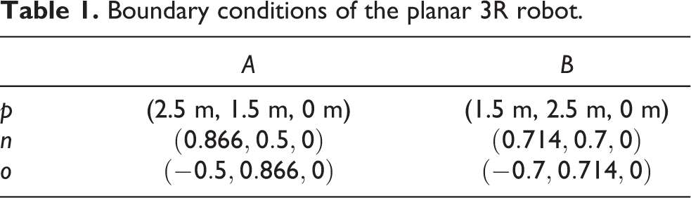
To simplify, assume that $l_{1} = l_{2} = l_{3} = 1$ m, and the robot moves linearly from the initial point A to the end point B. The values of A and B are shown in Table 1. A set of inverse kinematic solutions are shown in Table 2. As mentioned in Section 3.2, the parameter s is set to be dimensionless and ranges from 0 to 1. One can change the values and add a unit to the parameter.

Table 1.

Boundary conditions of the planar 3R robot.

	A	B
p	(2.5 m, 1.5 m, 0 m)	(1.5 m, 2.5 m, 0 m)
n	(0.866, 0.5, 0)	(0.714, 0.7, 0)
o	(−0.5, 0.866, 0)	(−0.7, 0.714, 0)

Table 2.

A set of inverse kinematic solutions of the planar 3R robot.

	A	B
s	0	1
θ₁ (rad)	0.258	0.970
θ₂ (rad)	0.583	0.380
θ₃ (rad)	−0.312	−0.574

The cubic polynomial interpolation is chosen to make a comparison to demonstrate the smoothness of the trajectory planned by the improved algorithm. To enhance the accuracy of the contour in the Cartesian space, we choose 11 via-points which uniformly distribute on the linear path. In order to obtain a smooth end-effector motion, the end-effector velocity is set to be constant at these via-points. The joint positions at the knots are obtained by the inverse kinematics. Cartesian velocities at the via-points are converted into joint velocities at the knots by using the inverse Jacobian. The trajectory segments between knots is calculated by interpolating cubic polynomials for each joint.

The trajectories and their velocities, accelerations and jerks of the end-effector obtained by the improved algorithm and the polynomial interpolation are compared in Figure 5. It is shown that the Cartesian path is accurate (see Figure 5(a)). The end-effector velocity, acceleration and jerk determined by the improved geodesic algorithm almost keep constant, but those obtained by the cubic polynomial interpolation oscillate obviously (see Figure 5.(b)). The maximum absolute value of position jerks for the end-effector of the geodesic trajectory is 0.042, while that of the polynomial trajectory is 41.901, as shown in Table 3. The end-effector orientation velocity, acceleration and jerk determined by the geodesic are almost constant, but those obtained by the cubic polynomial interpolation oscillate obviously (see Figure 5.(d)). The maximum absolute value of orientation jerks for the end-effector of the geodesic trajectory is 0.022, while that of the polynomial interpolation is 139.229 (see Table 3).

Figure 5.

The simulation results of the planar 3R robot in the Cartesian space: (a) the position; (b) the position velocity, acceleration and jerk; (c) the orientation; (d) the orientation velocity, acceleration and jerk.

Table 3.

Comparisons of maximum absolute jerk values.

	Joint			End-effector
Maximum absolute jerk	1	2	3	Position	Orientation
The geodesic algorithm	106.901	214.241	107.347	0.042	0.022
The polynomial interpolation	105.428	126.839	126.789	41.901	139.229

The trajectories, velocities, accelerations and jerks of the three joints are shown in Figure 6. The joint acceleration determined by the improved geodesic algorithm is smooth, but that obtained by the polynomial interpolation fluctuates. The fluctuation of the jerks planned by the polynomial interpolation is even more remarkable. The maximum absolute value of each joint jerk determined by both methods are given in Table 3. The jerk trajectory of each joint determined by the geodesic algorithm is continuous, but that obtained by the polynomial interpolation is discontinuous.

Figure 6.

The trajectory planning of the planar 3R robot in the joint space.

In both the Cartesian space and the joint space, the geodesic trajectory planning is smoother than the polynomial one. In the Cartesian space, the geodesic orientation is also smoother than that generated by the polynomial interpolation.

In addition, if we take d = (dp)² as the Riemannian metric, i.e.

\begin{array}{l} d = (d p)^{2} = (\begin{matrix} d θ_{1} & d θ_{2} & d θ_{3} \end{matrix}) D {(\begin{matrix} d θ_{1} & d θ_{2} & d θ_{3} \end{matrix})}^{T} \end{array}

Then, the elements of the coefficient matrix 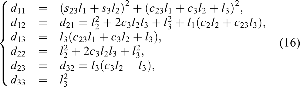$D = (d_{i j})_{3 \times 3}$ of the Riemannian metric will become

{\begin{array}{l} d_{11} & = & {(s_{23} l_{1} + s_{3} l_{2})}^{2} + {(c_{23} l_{1} + c_{3} l_{2} + l_{3})}^{2}, \\ d_{12} & = & d_{21} = l_{2}^{2} + 2 c_{3} l_{2} l_{3} + l_{3}^{2} + l_{1} (c_{2} l_{2} + c_{23} l_{3}), \\ d_{13} & = & l_{3} (c_{23} l_{1} + c_{3} l_{2} + l_{3}), \\ d_{22} & = & l_{2}^{2} + 2 c_{3} l_{2} l_{3} + l_{3}^{2}, \\ d_{23} & = & d_{32} = l_{3} (c_{3} l_{2} + l_{3}), \\ d_{33} & = & l_{3}^{2} \end{array}

In this case, it is easy to verify that |D| is zero, i.e. the coefficient matrix D is singular. Therefore, the Riemannian metric d = (dp)² cannot be applied to plan a linear motion for a planar 3R robot.

The improved geodesic algorithm for a spatial RRPP robot

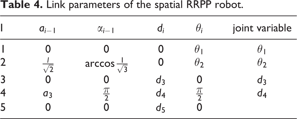
Consider the spatial RRPP robot shown in Figure 7. It is a simplified model of the XHK 5140 automatic tool-changing CNC vertical boring and milling machine tool with four DOFs. The first two joints are revolute joints, while the other two are prismatic. Its link parameters are shown in Table 4.

Figure 7.

A spatial RRPP robot.

Table 4.

Link parameters of the spatial RRPP robot.

I	a _i−1	α_i−1	d_i	θ_i	joint variable
1	0	0	0	θ ₁	θ ₁
2	$\frac{l}{\sqrt{2}}$	$\arccos \frac{1}{\sqrt{3}}$	0	θ ₂	θ ₂
3	0	0	d ₃	0	d ₃
4	a ₃	$\frac{π}{2}$	d ₄	$\frac{π}{2}$	d ₄
5	0	0	d ₅	0

The T matrix of the end-effector is

\begin{matrix} T & = & (\begin{matrix} n_{x} & o_{x} & a_{x} & p_{x} \\ n_{y} & o_{y} & a_{y} & p_{y} \\ n_{z} & o_{z} & a_{z} & p_{z} \\ 0 & 0 & 0 & 1 \end{matrix}) \end{matrix}

where

{\begin{array}{l} n_{x} = & \frac{\sqrt{2}}{\sqrt{3}} s_{1}, n_{y} = \frac{\sqrt{2}}{\sqrt{3}} c_{1}, n_{z} = \frac{1}{\sqrt{3}}; \\ o_{x} = & - c_{1} c_{2} + \frac{1}{\sqrt{3}} s_{1} s_{2}, o_{y} = - s_{1} c_{2} - \frac{1}{\sqrt{3}} c_{1} s_{2}, \\ o_{z} = & - \frac{\sqrt{2}}{\sqrt{3}} s_{2}; a_{x} = c_{1} s_{2} + \frac{1}{\sqrt{3}} s_{1} c_{2}, \\ a_{y} = & s_{1} s_{2} + \frac{1}{\sqrt{3}} c_{1} c_{2}, a_{z} = - \frac{\sqrt{2}}{\sqrt{3}} c_{2}; \\ p_{x} = & - \frac{s_{1} (s_{2} a_{3} - \sqrt{2} d_{3} - c_{2} d_{4})}{\sqrt{3}} + c_{1} (a_{1} + c_{2} a_{3} + s_{2} d_{4}) \\ + (\frac{c_{2} s_{1}}{\sqrt{3}} + c_{1} s_{2}) d_{5}, \\ p_{y} = & \frac{c_{1} (s_{2} a_{3} - \sqrt{2} d_{3} + s_{2} d_{4})}{\sqrt{3}} + c_{1} (a_{1} + c_{2} a_{3} + s_{2} d_{4}) \\ + (- \frac{c_{2} c_{1}}{\sqrt{3}} + s_{1} s_{2}) d_{5}, \\ p_{z} = & \frac{\sqrt{2} s_{2} a_{3} + d_{3} - \sqrt{2} c_{2} (d_{4} + d_{5})}{\sqrt{3}} \end{array}

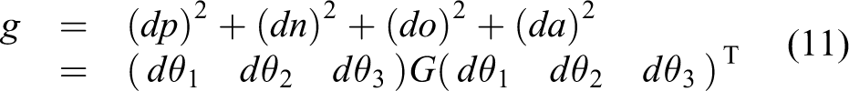
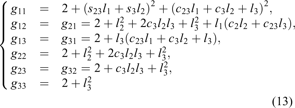
The Riemannian metric is given by

\begin{array}{l} g & = & {(d p)}^{2} + {(d n)}^{2} + {(d o)}^{2} + {(d a)}^{2} \\ = & (\begin{matrix} d θ_{1} & d θ_{2} & d d_{3} & d d_{4} \end{matrix}) G (\begin{matrix} d θ_{1} \\ d θ_{2} \\ d d_{3} \\ d d_{4} \end{matrix}) \end{array}

where $G = (g_{i j})_{4 \times 4}$ is the coefficient matrix of the metric, and its elements are

{\begin{array}{l} g_{11} = & \frac{1}{3} (6 + {(c_{2} a_{1} + a_{3} - \sqrt{2} s_{2} d_{3})}^{2} + {(s_{2} a_{1} + \sqrt{2} c_{2} d_{3} + d_{4} + d_{5})}^{2} + 2 (a_{1} + c_{2} a_{3} + s_{2} (d_{4} + d_{5} {))}^{2}), \\ g_{12} = & g_{21} = \frac{1}{\sqrt{3}} (2 + a_{3} (c_{2} a_{1} + a_{3} - \sqrt{2} s_{2} d_{3}) + (d_{4} + d_{5}) (s_{2} a_{1} + \sqrt{2} c_{2} d_{3} + d_{4} + d_{5})), \\ g_{13} = & g_{31} = - \sqrt{\frac{2}{3}} (a_{1} + c_{2} a_{3} + s_{2} (d_{4} + d_{5})), \\ g_{14} = & g_{41} = - \frac{c_{2} a_{1} + a_{3} - \sqrt{2} s_{2} d_{3}}{\sqrt{3}}, \\ g_{22} = & 2 + a_{3}^{2} + {(d_{4} + d_{5})}^{2}, g_{23} = g_{32} = g_{34} = g_{43} = 0, \\ g_{24} = & g_{42} = - a_{3}, g_{33} = g_{44} = 1 \end{array}

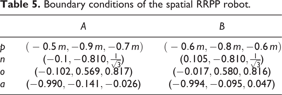
For simplicity, assume that $a_{1} = a_{3} = d_{5} = 1$ m, and the robot moves linearly from the initial point A to the end point B. The values of A and B are given in Table 5. A set of inverse kinematic solutions are shown in Table 6.

Table 5.

Boundary conditions of the spatial RRPP robot.

	A	B
p	(−0.5m, −0.9m; −0.7m)	(−0.6m, −0.8m; −0.6m)
n	( $- 0.1, - 0.810, \frac{1}{\sqrt{3}}$ )	( $0.105, - 0.810, \frac{1}{\sqrt{3}}$ )
o	(−0.102, 0.569, 0.817)	(−0.994, −0.095, 0.047)
a	(−0.990, −0.141, −0.026)	(−0.994, −0.095, 0.047)

Table 6.

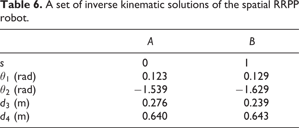
A set of inverse kinematic solutions of the spatial RRPP robot.

	A	B
s	0	1
θ₁ (rad)	0.123	0.129
θ₂ (rad)	−1.539	−1.629
d₃ (m)	0.276	0.239
d₄ (m)	0.640	0.643

Because the traditional geodesic algorithm is unsuitable for the trajectory planning of the RRPP robot, only the results planned by the improved geodesic algorithm are provided here. The trajectory and velocity, acceleration and the jerk of the end-effector are shown in Figure 8. The trajectories, velocities, accelerations and jerks of the joints are shown in Figure 9. The orientations of the end-effector are shown in Figure 10. It is shown that the geodesic trajectory is smooth in both the Cartesian space and the joint space. Therefore, the improved geodesic algorithm is effective in treating the spatial RRPP robot, which has four DOFs: two revolute and two prismatic.

Figure 8.

The trajectory planning of the spatial RRPP robot in the Cartesian space.

Figure 9.

The trajectory planning of the spatial RRPP robot in the joint space.

Figure 10.

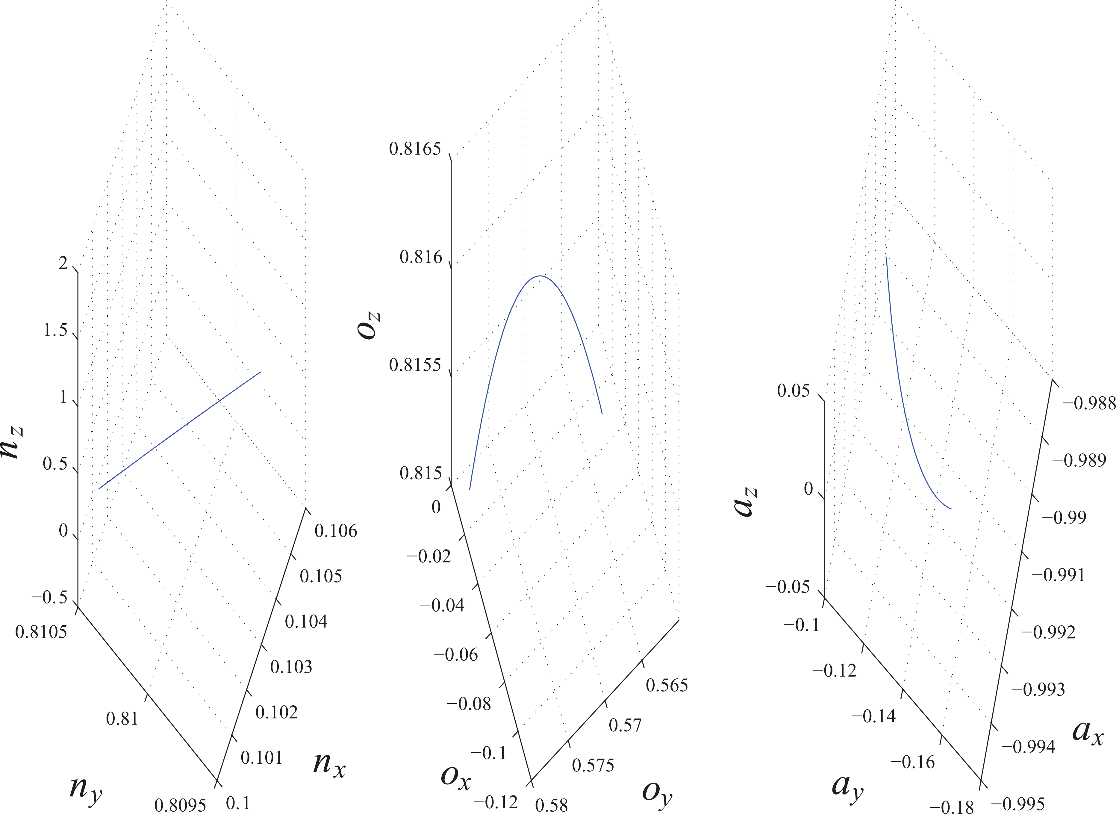
The planned orientation of the spatial RRPP robot in the Cartesian space.

Conclusion and future work

An improved geodesic algorithm is proposed for the trajectory planning of multi-joint robots. The geodesic trajectory planning has many advantages, but there still leave many fundamental problems unsolved such as orientation trajectory planning. The method can be used to tackle the orientation problem and can be applied to multi-joint robots. Smooth trajectories of robot end-effectors and joints are obtained. The joint variables are chosen to constitute a local coordinate system of the product of the positional space and the orientational space. By defining a new Riemannian metric that contains both the positional and rotational parameters, the traditional geodesic algorithm is improved so that it becomes capable of planning trajectories that include not only the position but also the orientation. Simulations are performed on the trajectory planning of both a planar 3R robot and another spatial RRPP robot, and it is demonstrated that the improved geodesic algorithm is effective in generating smooth motions for both the end-effector and the joints.

Finally, there is a limitation which is the present improved algorithm applies to robots with no more than six DOFs. In addition, the simulations provided in this paper only focus on linear motions. These are two limitations of the present work. Therefore, the future work will be directed to construct appropriate metrics to plan trajectories of robots with more than six or redundant DOFs, to achieve the geodesic planning of curvilinear motions, and to develop the control part.

Footnotes

Declaration of conflicting interests

The author(s) declared no potential conflicts of interest with respect to the research, authorship, and/or publication of this article.

Funding

The author(s) disclosed receipt of the following financial support for the research, authorship, and/or publication of this article: This work was supported by the National Key Technology R&D Program of China under Grant No. 2014BAF04B01.

References

Craig

. Introduction to Robots: Mechanics and Control, 3rd edn. Englewood Cliffs: Pearson/Prentice Hall, 2005.

Taylor

. Planning and execution of straight line manipulator trajectories. IBM J Res Development 1979; 23: 424–436.

Lin

Chang

Luh

JYS

. Formulation and optimization of cubic polynomial joint trajectories for industrial robots. IEEE Trans Automatic Control 1983; 28: 1066–1074.

Boryga

Graboś

. Planning of manipulator motion trajectory with higher-degree polynomials use. Mech Machine Theory 2009; 44: 1400–1419.

Piazzi

Visioli

. Global minimum-jerk trajectory planning of robot manipulators. IEEE Trans Indust Electron 2000; 47: 140–149.

Chettibi

Lehtihet

Haddad

Hanchi

. Minimum cost trajectory planning for industrial robots. Eur J Mech A Solids 2004; 23: 703–715.

Wang

Horng

. Constrained minimum-time path planning for robot manipulators via virtual knots of the cubic B-spline functions. IEEE Trans Automatic Control 1990; 35: 573–577.

Gasparetto

Zanotto

. A new method for smooth trajectory planning of robot manipulators. Mech Machine Theory 2007; 42: 455–471.

Žefran

Kumar

Croke

. On the generation of smooth three-dimensional rigid body motions. IEEE Trans Robotics Automation 1998; 14: 576–589.

10.

Zhang

Zhou

. Kuka youBot arm shortest path planning based on geodesics. In: Proceedings IEEE International Conference on Robotics and Biomimetics, 2013, pp. 2317–2321.

11.

Park

Ravani

. Bèzier curves on Riemannian manifolds and lie groups with kinematic applications. AMSE J Mech Design 1995; 117: 36–40.

12.

Kuffner

. Effective sampling and distance metrics for 3D rigid body path planning. In: Proceedings IEEE International Conference on Robotics and Automation, 2004, pp. 3993–3998.

13.

Noakes

Popiel

. Geometry for robot path planning. Robotica 2007; 25: 691–701.

14.

Gallot

Hulin

Lafontaine

. Riemannian Geometry. Berlin: Springer-Verlag, 2004.

15.

Tchoń

Dulba

. On inverting singular kinematics and geodesic trajectory generation for robot manipulators. J Intell Robotic Syst 1993; 8: 325–359.

16.

Selig

Ovseevitch

. Manipulating robots along helical trajectories. Robotica 1996; 14: 261–267.

17.

Zhang

Zhou

. Robot optimal trajectory planning based on geodesics. In: Proceedings IEEE International Conference on Control and Automation, 2007, pp. 2433–2436.

18.

Spivak

. A Comprehensive Introduction to Differential Geometry, Vol. 1. Berkeley, CA: Publish or Perish Press, 1979.

19.

Warner

. Foundations of Differentiable Manifolds and Lie Groups. New York: Springer, 1983.

20.

O’Meara

. Introduction to Quadratic Forms. Berlin: Springer-Verlag, 1973.

21.

do Carmo

. Differential Geometry of Curves and Surfaces. Englewood Cliffs, NJ: Prentice-Hall, 1976.

22.

Senlin

Yilong

. Submanifolds of product Riemannian manifold. Acta Math Sci 2000 20(B): 213–218.

An improved geodesic algorithm for trajectory planning of multi-joint robots