
Abstract
Real-time balance control of an eight-link biped robot using a zero moment point (ZMP) dynamic model is difficult to achieve due to the processing time of the corresponding equations. To overcome this limitation an intelligent computing technique based on Support Vector Regression (SVR) is developed and presented in this paper. To implement a PD controller the SVR uses the ZMP error relative to a reference and its variation as inputs, and the output is the correction of the angle of the robot's torso, necessary for its sagittal balance. The SVR was trained based on simulation data generated using a PD controller. The initial values of the parameters of the PD controller were obtained by the second Ziegler-Nichols method. In order to evaluate the balance performance of the biped robot, three performance indexes are used.
The ZMP is calculated by reading four force sensors placed under each of the robot's feet. The gait implemented in this biped is similar to a human gait, which is acquired and adapted to the robot's size.
The main contribution of this paper is the fine-tuning of the ZMP controller based on the SVR. To implement and test this, the biped robot was subjected to external forces and slope variation. Some experiments are presented and the results show that the implemented gait combined with the correct tuning of the SVR controller is appropriate for use with this biped robot. The SVR controller runs at 0.2 ms, which is about 50 times faster than a corresponding first-order TSK neural-fuzzy network.
1. Introduction
A biped robot has a leg structure similar to human anatomy. To be able to maintain its stability in dynamic situations such a robotic system requires a good mechanical design, force sensors to acquire the Zero Moment Point (ZMP) and the design of appropriate real-time controllers. Many such biped humanoid robots have been developed, including ASIMO by Honda, WABIAN 2R by Waseda University, HUBO KHR-3 by KAIST and QRIO by Sony. Vukobratović et al. have developed a mathematical model for a biped robot and its method of control [1]. Many researchers [2–4] have investigated the gait of biped robots based on human kinematic data; a particularly good study of the kinematics of a human body was done by Winter [5]. Because a biped robot is easily knocked down, to assure its dynamic stability Hirai et al. proposed a standard method for gait synthesis based on the ZMP [6]. Basically, this method consists of designing a desired ZMP trajectory, and afterwards, during the robot's motion, making on-line control corrections to the movement of the torso and pendulum to materialize the defined ZMP trajectory, based on the measurements of the force sensors on the feet.
For humanoid robotics, static walking is when the projection of the centre of mass (CoM) on the floor is always within the support polygon during the walking motion. The supporting polygon corresponds to the support foot in the single support phase, if flat contact with the ground is verified. In the double support phase the support polygon is the convex polygon inscribing the two parts of the feet that are touching the ground. In static walking the robot is always in static equilibrium, so it can stop its motion at any moment and does not fall down. Note that fast motion is not possible, since the dynamic couplings of the body parts could affect the static equilibrium. In stable dynamic walking the projection of the CoM on the floor is outside the supporting polygon during some phases of the gait. The ZMP, however, is always inside the support polygon. The equilibrium of the robot depends on the dynamics, and in general the motions performed are faster and smoother than with static walking [23].
Intelligent computing techniques have found wide application in the area of advanced control of biped robots, due to their strong learning and cognitive abilities and good tolerance to uncertainty and imprecision. To solve the biped robot's balance problem many researchers have been developing controllers using intelligent computing methods like fuzzy neural networks or neuro-fuzzy networks [12–14] and SVR [7, 17]. A survey of these techniques was undertaken by Katić et al. [15]. The control of a biped robot using the ZMP with an eight-link model is more accurate than methods based on a two-link model with mass concentrations, which is normally used for real-time balance control. In the two-link model, the active joint can either be the ankle [8–10] or the hip [11] to determine and apply the necessary torque for the robot's balance.
Sagittal balance control using an eight-link model is difficult to apply in real time due to the excessive computational effort. To overcome this problem a computational intelligence technique, the Support Vector Regression (SVR) technique, is used in this paper. The SVR is trained with the simulation data from an eight-link robot model and data generated by empirical rules based on the Ziegler-Nichols method [21]. As the ZMP control is nonlinear, an SVR is appropriate because it calculates the optimal hyper plane for the training data and is faster than a neural network. The SVR technique was initially developed by Vapnik [16]. Using the eight-link biped model together with one computational intelligence technique allows the real-time control of the biped robot with greater precision than using the biped robot's simplified two-link model.
In [26] the authors compared the SVR with a first-order Takagi-Sugeno-Kang (TSK) [25] neuro-fuzzy network controller using real experiments, and concluded that the SVR controller presents a slightly better (between 1% and 5%) stability than the neuro-fuzzy network. Also, the SVR controller runs at 0.2 ms, which is about 50 times faster.
The present work has the objective of improving the performance of the SVR controller. Three performance indexes are used to evaluate the performance of a biped robot's balance control method [7]. The main contribution of this paper is to use these performance indexes to fine-tune the initial proportional and derivative controller parameters obtained with the Ziegler-Nichols method, in order to achieve a better performance. This fine-tuning consists of correcting scale factors in the SVR inputs instead of changing the initial PD parameters in the simulator controller, with subsequent retraining of the SVR. The Ziegler and Nichols method [21] uses a set of empirical rules for tuning PID controllers based on experimental results of the system to be controlled.
The gait implemented in this biped robot is similar to a human gait, which was acquired and adapted to the robot's size [4, 22].
The experiments were performed with a biped robot, shown in Figure 1, that was designed and built at the Institute of Systems and Robotics, University of Coimbra, Portugal [7].

Implemented robot
2. Training data for the SVR
The method used to obtain the equilibrium of the robot in the sagittal plane consists of correcting the angle of the hips (torso) using the SVR [18–20] real-time output. Balance in the lateral plane is achieved by positioning the pendulum (θlateral) at its extreme lateral positions during the single phase. This way the lateral coordinate of the ZMP is neglected.
The SVR was trained with 239 uniformly distributed and normalized data points, and tested with another 68 data points [7], generated by simulation using a set of empirical rules proposed by Ziegler and Nichols [21].
The second Ziegler and Nichols method, the stability-limit method, sets the controller parameters based on an evaluation of the system at the limit of stability. Its first step is to determine experimentally the value of the critical proportional gain (Kc), defined as the smallest value of the controller gain that results in sustained oscillations when a pure proportional controller is used. The period of these oscillations is called the critical period of oscillation (Tc). The proportional parameter of the PD controller is Kp = 0.6·Kc and the derivative parameter (Td) is calculated from Tc, using the relationship Td= Tc/8.
The second Ziegler and Nichols method was applied for the biped robot system. In the experiment to determine Kc and Tc the robot was maintained with only one foot on the ground and the proportional controller gain was increased until the robot presented sustained oscillations, as shown in Figure 2.

XZMP and θtorso obtained at the limit of stability with the proportional controller active and Kc=10.3. The robot has only one foot on the ground.
The value of Kc obtained for the limit of stability was 10.3. Thus, Kp is 6.2, because Kp = 0.6Kc.
The critical frequency of oscillation (ωc) is equal to 2.7 rad·s−1, resulting in Kd equal to 1.8, because Kd = KpTd. Using this constant derivative, the training data and the testing data for the SVR were determined. The integral parameter was ignored to prevent oscillations of the torso.
The training data consisted initially of 34 pairs of points obtained by simulation [7] of the biped robot model with steps of four seconds (seven points for each of five step lengths, excluding the pair (EXZMP, Δθtorso) = (0, 0)). For each of the previous 34 pairs, eight new pairs of points were generated with DXZMP

The first term of this equation is Δθtorso k, obtained by simulation of steps taking four seconds [7].
The following values were obtained: 307 (34×9+1), 239 (34×7+1) of those used for training and 68 (34×2) for testing the SVR.
3. Real-Time Control Strategy
The control strategy is one of the most important issues in controlling a biped robot. Many control strategies are available and may be based on fuzzy systems, neural networks, classic control, support vector machines, and hybrid systems.
The main blocks of our biped robot control are presented in Figure 3. The control system block is implemented by an SVR controller.
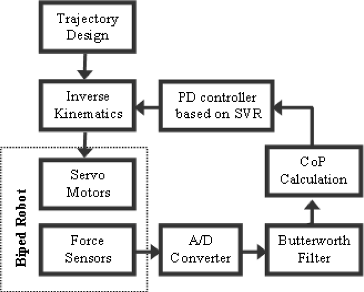
Balance control strategy of the biped robot
For real-time control, the actual value of the ZMP is needed. When the ZMP is within the stable region, the ZMP is equal to the centre of pressure (CoP) [24]. To determine the CoP, four force sensors are implanted under each foot of the robot. The CoP is calculated by

where Fi is the measured force in sensor i, and r̂ i is the position vector.
The force sensors' values are acquired by an analogue to digital converter (ADC) with 10-bit resolution and a maximum 30 Hz sampling rate. The force measurements are noisy because the force sensors are sensitive to vibrations during motion, so a second-order Butterworth low-pass filter is used to remove the high-frequency noise from the force sensor signals. A cut-off frequency of 3 Hz was set.
4. Experimental Results of Tuning
The choice of the proportional and derivative parameters of the controller was based on the Ziegler-Nichols method, but these parameters needed to be refined in order to optimize system performance. To refine the parameters the entries of the SVR (EXZMP and DXZMP) are adapted by the gain factors FP and FD, which indirectly influence the proportional and derivative terms, respectively.
The factors used in the experiments and the results of these experiments are presented in Tables 1 and 2. In the experiments the robot was walking (0.07 m) on a flat horizontal surface, using the trajectories of the human gait, dragging a mass of 1.5 kg (providing an effective pulling force about 5 N), as Figure 4 shows. Figure 5 shows the behaviour of the main variables of the biped robot during four steps. The values presented in this figure were normalized such that the unit values correspond to 25 degrees for θtorso, 10 degrees for θankle, 55 degrees for the pendulum lateral angle (θlateral) and 0.047 m for XZMP. In the figure it can be noticed that the θtorso is deviated forward relative to the θtorso D in order to keep the sagittal balance and XZMP near zero (XZMPref =0).

Snapshots of one step walked on a horizontal flat surface pulling a mass with SVR control active

XZMP, XZMPref, designed torso (θtorsoD), torso and lateral angles when the robot walks on a horizontal flat surface pulling a mass with SVR control active
Performance indexes - derivative case, experiments with a mass

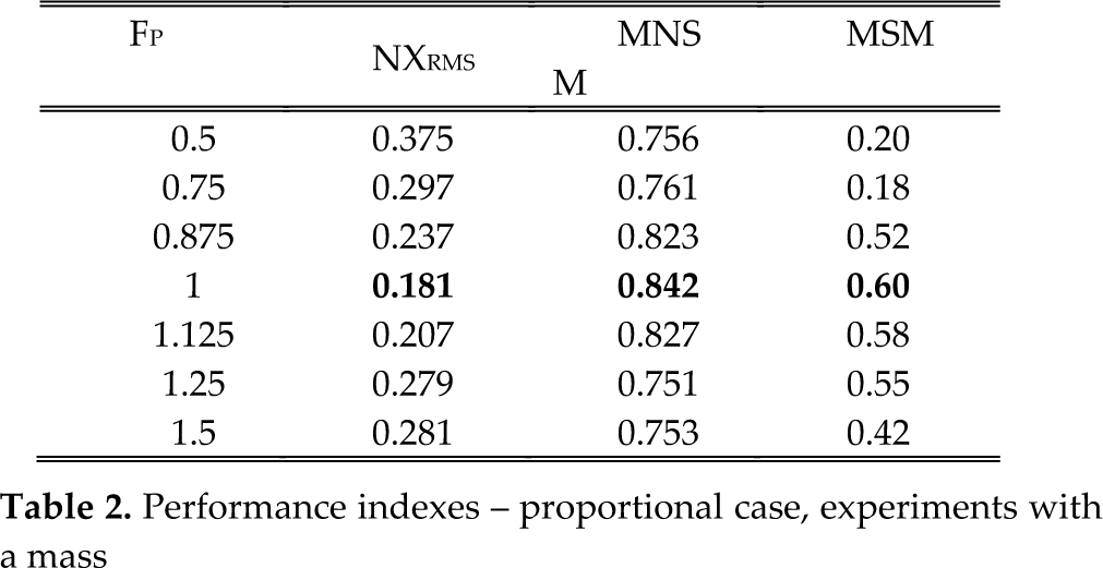
Performance indexes – proportional case, experiments with a mass
The time of the swing phase of the step is about two seconds, which represents a step time of about four seconds. The implemented step time is about five seconds (three seconds for the double phase), due to the need to perform the lateral control (the pendulum must move from 50 to −50 degrees or vice versa).
To determine which are the best parameters for the PD controller, and because the result plots are inconclusive, three performance indexes are proposed. The first is the normalized root mean square of XZMP - XZMP_ref (NXRMS); the second is the mean of the normalized stability margin (MNSM) and the third is the minimum of stability margin (MSM). These indexes were calculated for four walking steps and are described by
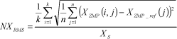
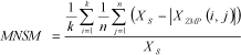

where k is the number of steps, n is the number of the force sensor samples and Xs is the X absolute coordinate of the force sensor locations, which corresponds to the maximum possible value of XZMP (in our robot, this is 0.047 m). The optimal value for NXRMS is zero and for both MNSM and MSM it is one.
Tables 1 and 2 present the three performance indexes' values for the experiments. The best values are highlighted in bold. The results in Table 2 were obtained with FD = 1.25.
The experiments show that the derivative controller parameter should be altered by the factor 1.25, and the proportional by 1. Since the proportional factor exhibits its best performance when FP = 1, there is no need for more iterations to find another FD.
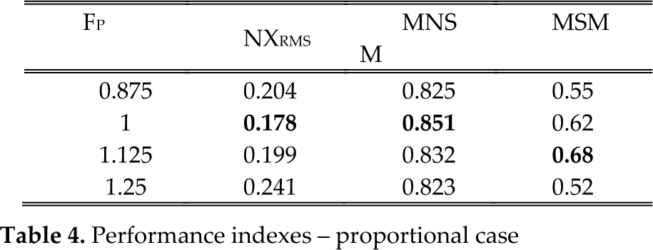
Experiments with the robot without external disturbances were also performed to verify the correctness of the factors. Tables 3 and 4 give the results of these experiments, confirming the previous factors, although the MSM index indicates FP=1.125 as the best.
Performance indexes – derivative case

Performance indexes – proportional case
Experiments with variation of the inclination slope were performed, using the initial and the improved SVR controller. In the following experiments the robot's right foot was placed in the air in an ascending (see Figure 8) and descending (see Figure 11) slope. The ascending slope was varied continuously during 10 s, from 0 to 10 degrees and again to 0 degrees using the initial (see Figure 6) and the improved (see Figure 7) SVR controller. The descending slope was varied continuously during 8.5 s, from 0 to −10 degrees and again to 0 degrees using the initial (Figure 9) and the improved (Figure 10) SVR controller.
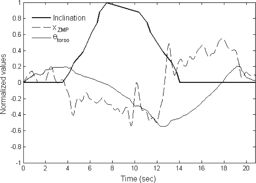
XZMP and θtorso when the robot is standing with one leg in the air; the slope varies from 0 to 10 degrees and 10 to 0 degrees with the initial SVR controller

XZMP and θtorso when the robot is standing with one leg in the air and the slope varies from 0 to 10 degrees and 10 to 0 degrees, with the improved SVR controller

Snapshots of the behaviour of the robot when it is standing with one foot in the air and the slope varies from 0 to 10 degrees and 10 to 0 degrees, with the improved SVR controller
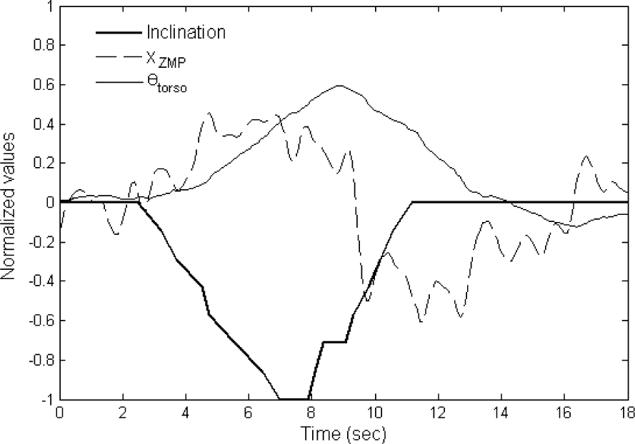
XZMP and θtorso when the robot is standing with one leg in the air, and the slope varies from 0 to −10 degrees and −10 to 0 degrees, with the initial SVR controller
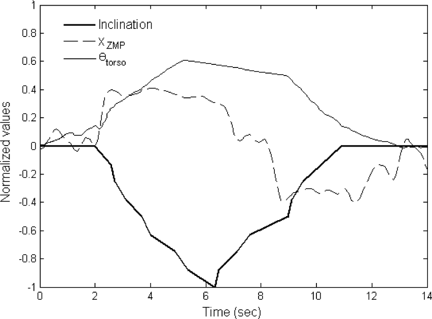
XZMP and θtorso when the robot is standing with one leg in the air and the slope varies from 0 to −10 degrees and −10 to 0 degrees, with the improved SVR controller

Snapshots of the behaviour of the robot when it is standing with one foot in the air and the slope varies from 0 to −10 degrees and −10 to 0 degrees, with the improved SVR controller
Again, the values shown in figures 6, 7, 9 and 10 are normalized with the constants used previously. The inclination of the slope is normalized by dividing by 10. The value of the slope of the ramp was obtained using the images from a digital video camera.
In the slope experiments it can be seen that the initial SVR controller keeps the XZMP between −0.6 and 0.6. In the improved SVR controller the values of XZMP are lower (between −0.4 and 0.4), increasing the stability of the robot.
5. Conclusions
The real-time control of a biped robot using the dynamic model of the ZMP is difficult to achieve because of the time required to process the corresponding equations.
An SVR balance controller allows the real-time control of the robot using an eight-link biped model. The controller uses the real ZMP, acquired by force sensors placed under the robot's feet. The control method was tested and satisfactory results were obtained.
The biped robot did not fall in any of the experiments with the balance controller active, and it kept a good stability margin, thereby demonstrating that the SVR controller is a good solution for biped robot balance control.
Three performance indexes were used to fine-tune the PD parameters using gain factors. It was shown that the gain factors obtained improve the performance of the robot.
In future work, we intend to use other recent computational intelligence control methods, like the extreme learning machine, and compare the results obtained with the SVR and with other classic methods.
6. Acknowledgments
The authors would like to thank the Portuguese Fundação para a Ciência e a Tecnologia for financial support.