
Abstract
An optimal calibration method for a micro-electro-mechanical inertial measurement unit (MIMU) is presented in this paper. The accuracy of the MIMU is highly dependent on calibration to remove the deterministic errors of systematic errors, which also contain random errors. The overlapping Allan variance is applied to characterize the types of random error terms in the measurements. The calibration model includes package misalignment error, sensor-to-sensor misalignment error and bias, and a scale factor is built. The new concept of a calibration method, which includes a calibration scheme and a calibration algorithm, is proposed. The calibration scheme is designed by D-optimal and the calibration algorithm is deduced by a Kalman filter. In addition, the thermal calibration is investigated, as the bias and scale factor varied with temperature. The simulations and real tests verify the effectiveness of the proposed calibration method and show that it is better than the traditional method.
1. Introduction
Nowadays, the progress in micro electro-mechanical systems (MEMSs) has enabled the development of low-cost inertial measurement units (IMUs), which are increasingly used in biomedical applications [1], in robots' navigation systems [2] and in microsurgical instruments [3]. However, the performance of MEMS inertial sensors is degraded by fabrication defects, including produced asymmetric structures, the misalignment of actuation mechanisms and deviations of the centre of mass from the geometric centre. The inner factors cause output errors, which are often divided into deterministic and random errors [4]. Moreover, the inertial measurement unit integrated by MEMSs' inertial sensors (MISs) may still contain IMU package misalignment errors and IMU sensor-to-sensor misalignment errors [4]. Therefore, it is essential to develop an effective calibration method to reduce the errors and increase the MIMU's precision and stability.
The method most commonly used for the calibration of MEMS accelerometers is the six-position method [5], which requires the inertial system to be mounted on a levelled surface with each sensitivity axis of each sensor pointing, alternately, up and down. This calibration method can be used to determine the bias and scale factors of the sensors, but cannot estimate the axes misalignments or non-orthogonalities. The multi-position calibration method is proposed to detect more errors [6]. These methods depend on the earth's gravity as a stable physical calibration standard. Furthermore, some special apparatus, such as motion sensing equipment [7] and robotic arms [8–9], are used for calibration. For the calibration of low-cost MEMS gyroscopes, the Earth's rotation rate is smaller than its resolution. Therefore, the traditional calibration method is dependent on a mechanical platform, rotating the IMU into different, predefined, precisely-controlled orientations and angular rates. Such a method was primarily designed for in-lab tests, which often require the use of expensive equipment [5]. Therefore, some calibration methods that do not require the mechanical platform have been proposed. In [10], an optical tracking system is used. In [11], an affordable three-axis rotating platform is designed for the calibration. Meanwhile, schemes for in-field user calibration without external equipment are proposed. Fong et al. [12] calibrated gyroscopes by comparing the outputs of the accelerometer and the IMU orientation integration algorithm after arbitrary motions, which requires an initial rough estimate of the gyroscope's parameters. Jurman [13] and Hwangbo [14] proposed a kind of shape-from-motion calibration method with magnitude constraint of motion. Furthermore, the calculation algorithm is another important issue. The calibration parameters are computed by the algorithm. The least squares method is the algorithm most commonly used in scalar calibration to estimate the calibration parameters [6, 11–14]. H.L Zhang et al. [15] implemented an optimal calibration scheme by maximizing the sensitivity of the measurement norms with respect to the calibration parameters. The algorithms typically lead to a biased estimate of the calibration parameters and may give non-optimal estimates of the calibration coefficients. To avoid this, Panahandeh et al. [16] solved the identification problem by using the maximum likelihood estimation (MLE) framework, but only simulation results are presented. In fact, the biases and scale factors vary with temperature. The thermal calibration is also an indispensable process for MIMU. However, the literature seldom completes this type of calibration.
In this paper, an optimal calibration method for a MIMU is presented. Firstly, the measurement noise of the sensors is analysed to provide the information for the calibration. Next, the concept of the calibration method is introduced, which consists of a calibration scheme and a calibration algorithm. The optimal calibration scheme is designed by the D-optimal method [17–18]. Meanwhile, the optimal calibration algorithm is deduced by a Kalman filter. The calibration parameters, like scale factors, misalignments and biases, are estimated. Afterwards, thermal calibration is implemented to determine the scale factors and biases in different temperatures. In the end, the results of the simulations and experiments verify the effectiveness of the proposed method, and the performance of the MIMU is improved after the calibration.
The paper is organized as follows. Section 2 presents the hardware of the MIMU and introduces the inertial sensor model. Section 3 describes the character of the sensors' measurement noise, and the overlapping Allan variance is applied. Section 4 gives the MIMU model, where the scale factors, package misalignments, sensor-to-sensor misalignments and biases of the accelerometer and gyroscope triads are considered as the calibration parameters. Then, the optimal calibration algorithm for the gyroscope triad and the accelerometer triad is proposed, followed by the optimal calibration scheme designed by the D-optimal method. The thermal calibration of the MIMU is presented at the end of the section. Section 5 reports the calibration results of MIMU through both simulations and real tests. It shows that the improved multi-position approach outperforms the traditional calibration method. Conclusions are drawn in section 6.
2. Hardware description
A MIMU has been constructed by using MEMS gyros and a MEMS accelerometer. A MMA7260 accelerometer measures the triple-axis acceleration; three single-axis ADXRS300 gyros measure the angular rate in yaw, roll and pitch. Finally, the printed circuit boards (PCBs) of the x, y gyros are kept orthogonal by a slot.
The dynamic range of the ADXRS300 gyro is ±300°/s [19], and full range-scale of the MMA7260QT accelerometer is ±1.5 g [20]. The outputs from the sensors are analogue voltages that are proportional to the inputs as the rotation rate or acceleration. At zero input, the nominal output of the sensor is bias; positive rotation (clockwise) or acceleration increases the voltage from the nominal null offset value, whereas negative rotation (anticlockwise) or deceleration decreases the voltage output. The null offset value must be subtracted from the raw sensor output measurements. The specifications of the sensors are shown in Table 1.
The specifications of the sensors

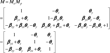
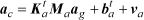
Based on the above analysis, the output of acceleration measured by the accelerometer can be described by the following equation:

where Va is the voltage of acceleration, a is the true acceleration, ba is the sensor bias, Ka is the scale factor (or acceleration gain) and εa is the sensor's noise.
A similar equation can be used to describe the angular velocity measured by the gyros on the single axis:

where V
Although the MEMS gyro's and MEMS accelerometer's parameters are given in the manuals, a dynamic range modification of the MEMS sensors exists. The errors of the parameters as biases and scale factors are deterministic errors, which are reduced by calibration. In addition, the random errors are measurement noises, which should not be ignored in calibration. Therefore, the noise needs to be characterized. For this unit, the data were collected using a multifunction 12-b data-acquisition card from National Instruments, the DAQCard-6008, which is controlled by a script based on National Instruments' LabVIEW 2007.
3. Analysis of the measurement noise
Several variance techniques have been devised for the stochastic modelling of the random errors. These are basically very similar and primarily differ in that various signal processing - by way of weighting functions, window functions, etc. - are incorporated into the analysis algorithms in order to achieve a desired result for improving the model characterizations. The simplest is the Allan variance.
The Allan variance is a method of representing the root mean square (RMS) random drift error as a function of averaging time. It is simple to compute and relatively simple to interpret and understand. The Allan variance method can be used to determine the characteristics of the underlying random processes that give rise to the data noise. This technique can be used to characterize various types of error terms in the inertial-sensor data by performing certain operations on the entire length of data.
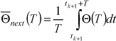
Assume that there are N consecutive data points, each having a sample time of t0. Forming a group of n consecutive data points (with n < N / 2), each member of the group is a cluster. Associated with each cluster is a time T, which is equal to nt0. If the instantaneous output rate of the inertial sensor is Θ(T), the cluster average is defined as:

where
The definition of the subsequent cluster average is:
where tk+1 = tk + T.
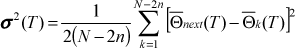
Performing the average operation for each of the two adjacent clusters can form the difference:

For each cluster time T, the ensemble of
Obviously, for any finite number of data points (N), a finite number of clusters of a fixed length (T) can be formed. Hence, equation (6) represents an estimation of the quantity
In addition, the percentage error is equal to:

where N is the total number of data points in the entire run and n is the number of data points contained in the cluster.
Equation (7) shows that the estimation errors in the region of a short cluster length T are small where the number of independent clusters in these regions is large. In contrast, the estimation errors in the region of a long cluster length T are large where the number of independent clusters in these regions is small. In order to avoid the estimation error increasing due to a lack of samples, the overlapping Allan variance was proposed [22] The use of overlapping samples improves the confidence of the resulting stability estimate. The formula is expressed as follows:
where m is the averaging factor.
The static data from the MIMU were collected with a sampling rate of 1000 Hz at room temperature 25°C. By applying the overlapping Allan-variance method to the whole data set, a log–log plot of the overlapping Allan standard deviation versus the cluster time is shown in Figure 1 for the accelerometers data and Figure 2 for the gyros data. As shown in these figures, the drift characteristic of the sensors is at its worst as

Accelerometers overlapping Allan variance results

Gyros overlapping Allan variance results
In dealing with the sensor signals over a period of time determined using the Allan variance analysis above, it will keep the bias drift minimal during the successive time period when the calibration data are collected. Accordingly, the white noise is only considered in the calibration.
4. Calibration method
Calibration is the process of comparing the instruments output with known reference information and determining the coefficients that force the output to agree with the reference information over a range of output values [23]. Moreover, many researchers [5–16] have developed calibration methods for the IMU. Before the description of our own calibration method, a clear concept of the calibration method is introduced first of all. The calibration method of the IMU should consist of two aspects, which are a calibration scheme and a calibration algorithm. The scheme is to design the experiments, while the algorithm is to compute the parameters by the experimental data. A novel calibration method is presented in this section according to this concept.
Firstly, the complete calibration model of the MIMU is described. Next, an optimal calibration method is proposed by an optimal calibration scheme and an optimal calibration algorithm. The scheme is the design of a calibration experiment for the gyroscope triad and the accelerometer triad, and the calibration results are computed by the optimal algorithm. Finally, thermal calibration is described.
4.1 Calibration model
The measurement model of the accelerometer or gyroscope generally includes bias, scale factors and random error. Bias and scale factors are considered as the most significant parameters, which change with different temperatures. It is also a very important characteristic for inertial sensors (though this is dealt with by independent thermal calibration, as explained at the end). In this section, the calibration procedure is performed at a stable temperature and the self-heating effects can be ignored, as the MIMU is calibrated after the sensors are warmed up to thermal stability. Moreover, the random error can be considered as white Gaussian noise from the last section.
In this paper, the MIMU consists of three almost orthogonally mounted gyroscopes and a three-axis accelerometer. As to the unit, the misalignment error would be induced because of the sensors' installation. The misalignment error is divided into two sources: package misalignment error and sensor-to-sensor misalignment error. Package misalignment error is defined as the angle between the true axis of sensitivity and the body axis of the package. Sensor-to-sensor misalignment error defines the misalignment error due to the non-orthogonality of the IMU's axes.
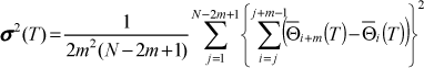
The package misalignment angle can be defined as three angles. First, for a rotation about the z -axis by an angle of
Second, for a rotation about the y -axis by an angle
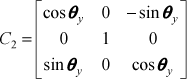
And finally, for a rotation about the x -axis by an angle of

The three angles can be considered as small angles. Then, the package misalignment error can be represented by the following equation:
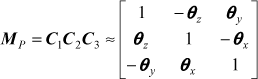
The sensor-to-sensor misalignment error or non-orthogonality can be also considered as creating a series of rotation matrices that define the relationship of the misaligned axes to those of the perfectly orthogonal triad. Generally, it is considered that the axes x of the frames coincide and - assuming small angles - the non-orthogonality matrix can be approximated by:

Then, the total misalignment error can be written as:
Consequently, the measurement of the accelerometer cluster can be expressed as:
where

where kia and bia, respectively, denote the scale factor and the bias of the i th accelerometer output, i = x,y,z. The misalignment matrix of the accelerometer is written as:

Analogously, the measurement of the gyroscope cluster can be written as:

where
The misalignment matrix of the gyroscope triad is written as:

The task of MIMU calibration is to estimate such parameters as scale factors, misalignments, biases of the accelerometer and the gyroscopes. Meanwhile, the experiment is implemented at 25°C in the lab. The key technology of the calibration can be divided according to two aspects: the calibration scheme and the calibration algorithm. We will discuss these separately in the following sections.
4.2 Calibration scheme
The calibration scheme is the experiment design for the MIMU. Generally, a multi-position calibration scheme is used for the IMU's calibration. The general principle of the method is to design enough positions to estimate the calibration parameters. At least 12 different equations for determining (that is, at least 12 positions for the MIMU) are required in calibration, as there are 12 unknown parameters in both the accelerometer triad and the gyroscope triad. In order to avoid computational singularity in estimation, more positions are desired to get numerically reliable results in reality. Afterwards, the question as to how the positions are designed in calibration arises. The current literature has seldom discussed in detail how the positions are optimized - in other words, the scheme not only makes all the calibration parameters identifiable, but also maximizes their numerical accuracy. In the current context, the optimal calibration positions are proposed by the D-optimal method.
According to equations (15)–(17), the following equation can be deduced:

where
By rearranging equation (19), we can attain the following equations:
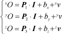
where
iO denotes the MIMU's measurement of the i axis, i=x,y,z.
Assume Ξ is an experimental procedure, which is used to calibrate the parameters in equation (20). The experimental procedure is composed of n tests, defined as Uk (k ∈ [1,n). Each test Uk corresponds to a test position of Ξ, which is generated by the input vector Γk = [
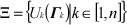
with associated outputs i O.
It is shown that a D-optimal design can be achieved with p ≤ n ≤ p(p + 1)/2, where p is the number of parameters to be estimated. From equation (21), one can see that there are four unknown parameters for each output axis, so the optimal number of measurement positions must exist in [5,13].
Then, the optimal function can be described as follows:

where
In addition, the procedure of D-optimal design is described as follows:
Select n test positions from global candidate positions and calculate the object function Select a maximum n ≤ 12,return to step 1) Optimal experiment positions Ξ*
Four optimal positions for each iO are acquired; therefore, totally, 12 optimal positions can be attained for calibration. Then, there are the duplicate positions. After removing the duplicate positions, the nine optimal positions (which are listed in Table 2) are used for calibration. It is noticed that the MEMS gyros in the paper are low cost and cannot measure the Earth's rotation rate. Therefore, a rotation rate table is used in the calibration to produce a reference signal. Meanwhile, gravity is also considered as a reference signal.
Optimal positions for calibration

4.3 Calibration algorithm
The calibration algorithm is the computation of the calibration parameters from the data, which is collected by the calibration scheme. Because the collected data from the MIMU contain random noise, the optimal estimate algorithm is generally adopted. The least squares algorithm is the most commonly used in estimating the calibration parameters. The algorithms typically lead to a biased estimate of the calibration parameters and may give non-optimal estimates of the calibration coefficients. Consequently, a Kalman filter is designed for the calibration algorithm in what follows.
4.3.1 Kalman filter design
A Kalman filter (KF) eliminates random noise and errors using knowledge about the state-space representation of the system and uncertainties in the process: the measurement noise and the process noise. As such, it is very useful as a signal filter in the case of signals with random disturbances or else when signal errors can be treated as an additional state-space variable in the system. For linear Gaussian systems, the Kalman filter is the optimal minimum mean square error estimator.
The model can be expressed as follows:
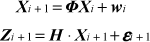
where
Moreover, the Kalman filter can be derived by the following process:
Time updating:

Measurement updating:
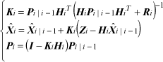
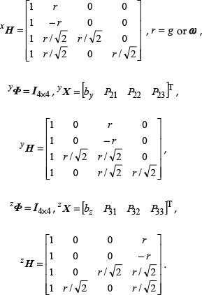
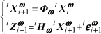
According to the optimal positions, a bank of Kalman filters is deduced:

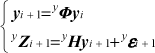

where
x
Three simpler Kalman filters have been designed for the MIMU calibration. Next, the observability is analysed to make sure that the calibration parameters are identifiable.
According to [24], the n -state discrete linear time-invariant system has the observability matrix G defined by:
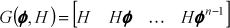
The system is observable if, and only if, rank(G) = n. We can derive the following equations from equations (26)–(28)

Because
i
Therefore, the scale factors, biases and orthogonalization angles of the MIMU are estimated by the three Kalman filters. However, the scale factors and biases are not stable in different temperatures. Therefore, thermal calibration is also important for the MIMU.
4.4 Thermal calibration
The purpose of thermal calibration is to reduce the errors caused by the variation of the scale factors and biases of the MIMU when operated under different temperatures. There are two main approaches for thermal testing [5]: (1) Allow the IMU enclosed in the thermal chamber to stabilize at a particular temperature corresponding to the temperature of the thermal chamber and then record the data (this method of recording the data at specific temperature points is called the ‘Soak method’). (2) In the so-called ‘thermal ramp’ method, the IMU temperature is linearly increased or decreased for a certain period of time. We would use the Soak method to investigate the thermal effect of the sensors.
According to equation (15) and equation (17), the model of thermal calibration can be described:

where
and
The misalignment parameters can be obtained by the last section and they are not varied by the temperature, so only the scale factors and biases should be estimated. The calibration scheme can be designed by no. 1–6 in Table 2.
Analogously, the calibration algorithms are deduced:

where

It is noticed that the variances of the MIMU measurements are different for different temperatures, and so the covariance matrices of the measurement noise should be calculated for different temperatures. In thermal calibration, a turntable and a thermal chamber are assembled together to form a thermal-turntable unit, as shown in Figure 3.

The thermal test setup
5. Calibration Results
5.1 Simulation and calibration results
In order to verify the calibration method, a Monte Carlo simulation is first implemented. The true values of the 12 parameters in the calibration model are listed in Table 3. It is noted that the parameters are dimensionless parameters.
The simulation parameters

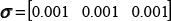
These parameters used in the simulation were chosen to be within the range of the expected MIMU parameters. The sensor noise standard deviation is:
Both the traditional method and the proposed approach were performed in the simulation. It is noted that the traditional method is the method of least squares [5]. The results are shown in Figures 4–7.

The bias errors of the two calibration methods
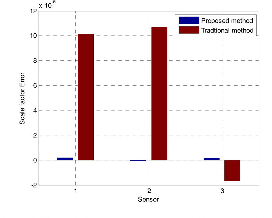
The scale factors error of the two calibration methods
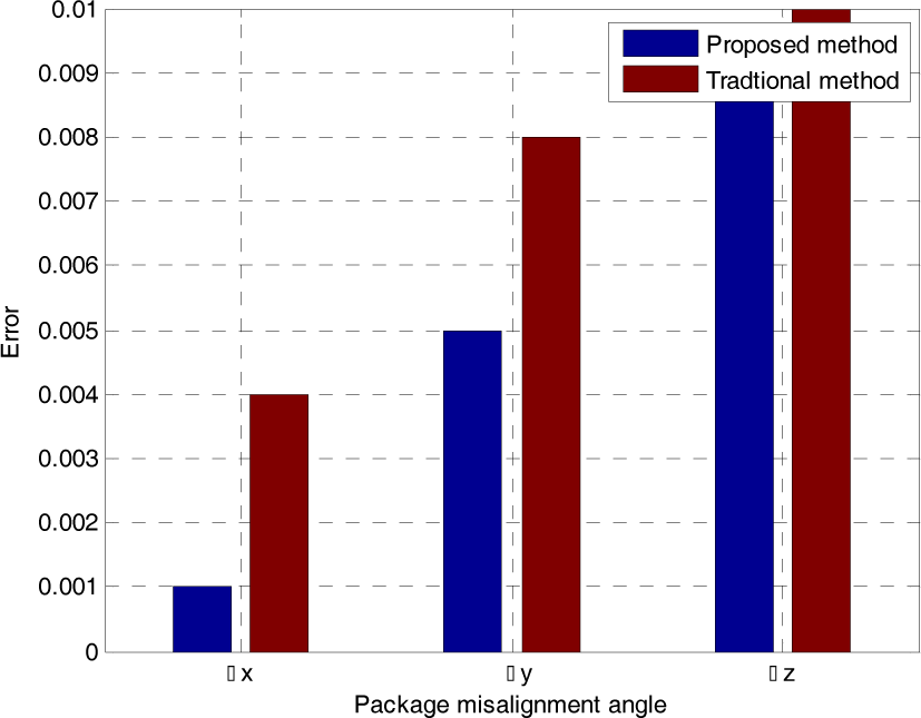
The package misalignment angle errors of the two calibration methods
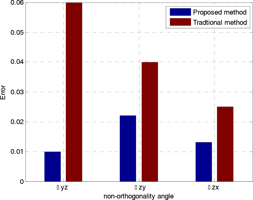
The orthogonalization angle errors of the two calibration methods
The parameters' errors are smaller under the proposed method. Meanwhile, we find that parameters estimated by the traditional method will deviate significantly when the noise standard deviation is increased. However, the proposed method is still effective.
The simulation results have shown the performance of the filter and the accuracy of the proposed method. Next, the MIMU is calibrated in the lab, using a cube and a rate table. The outputs were sampled at a rate of 1000 Hz and the LabVIEW program stored the digitalized analogue measurements from the MIMU. The collected data were later read into the MATLAB program for processing. The calibration results are shown as follows. Figures 8–11 show the parameters of the three-axis accelerometers while the gyros' are shown in Figures 12–15.
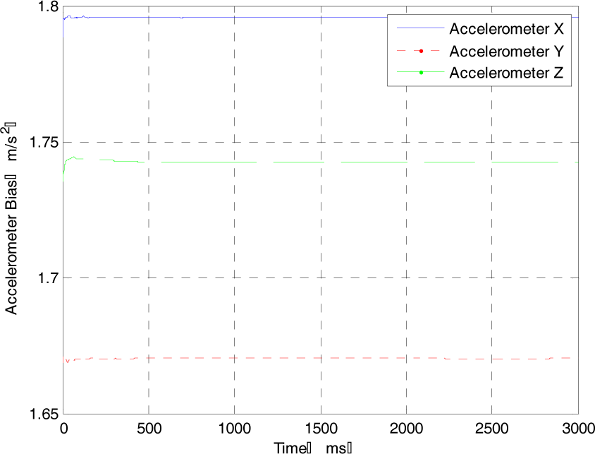
Bias of the accelerometers

Scale factor of the accelerometers

Package misalignment angles of the accelerometers

Non-orthogonality angles of the accelerometers

Bias of the gyros

Scale factor of the gyros

Package misalignment angles of the gyros
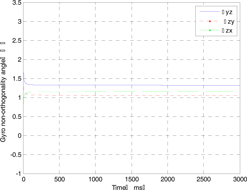
Non-orthogonality angles of the gyros
The estimated results are listed in Table 4. It indicates that the estimating procedure is convergent and it takes less than two seconds to complete. The parameters converge quickly to the stable values.
The calibration results of the MIMU

5.2 Thermal calibration results
The temperature of the thermal chamber varies from 0°C to 50°C. A total of nine different temperatures are considered in this experiment. For each temperature, the MIMU is allowed to stabilize before recording data.
We calculate the variances of the MIMU measurements at different temperatures. The results are listed in Table 5, and they are different for the different temperatures. The scale factors and biases for the MIMU at different temperatures are shown in Figures 16–19. We can see that the biases and scale factors of the MIMU vary significantly with temperature. Hence, it is necessary to get the thermal calibration model for low-cost MEMS sensors to compensate for these biases and scale factor drift with temperature.
The measurement variance for different temperatures


Variation of the accelerometer scale factor with temperature

Variation of the accelerometer biases with temperature

Variation of the gyroscope scale factor with temperature
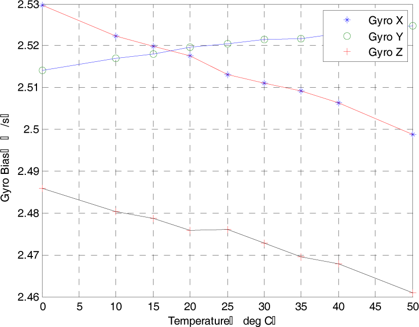
Variation of the gyroscope biases with temperature
To evaluate the performance of the proposed calibration method, we compare it with the six-position method used in [5] which is the most commonly used. This requires the IMU to be mounted on a levelled table with each sensitive axis pointing alternately up and down. For a triad of orthogonal sensors, this results in a total of six positions. The thermal calibration is implemented by the traditional method for the same temperature. Next, the calibrated measurements of the static IMU are compared by two calibration methods. The results are shown in Figures 20–21. By comparison with the traditional method, the proposed method can improve the measurement precision by an order of magnitude.

The measured accelerations with zero-inputs

The measured angular velocities with zero-inputs
5.3 Discussion
Light-weight and low-cost MIMUs are widely used. However, these units need calibration for an accurate measurement solution. The computed biases, scale factors, package misalignment angles and sensor-to-sensor misalignment angles are estimated in a stable temperature through the optimal calibration method. By observing the estimated parameters of the MIMU, we can find out the differences between sets of sensors, even though they belong to the same type. In fact, the parameters' values are not identical to the specifications' values. Meanwhile, it is evident that the accelerometer triad contains smaller orthogonalization errors than the gyros, since the accelerometer triad consists of one three-axis sensor while the gyroscope triad has three single-axis sensors, which are not easy to install orthogonally.
We get the misalignment angles in the optimal calibration at a stable temperature, and then estimate the biases and scale factors of the MIMU at different temperatures by thermal calibration. The experiments have shown that the random errors' variances of the measurements are different. It is useful for the estimation of the biases and scale factors by the Kalman filter. As observed in Figure 17 and Figure 19, there is an almost linear relationship between the biases and temperatures. Hence, a linear interpolation formula can be deduced for calibration in the temperature range. As observed from Figure 16 and Figure 20, the scale factors have an ambiguous relationship with temperature, but the interpolation polynomial can be obtained. The temperature drift errors can be reduced by thermal calibration.
6. Conclusion
The calibration of MIMU is an important phase in improving performance. This paper has presented an optimal calibration method for the MIMU, together with deduction, simulation and experimental results. We analyse the random errors by overlapping Allan variance, and the white noise is taken account of by the calibration. The general calibration model includes such calibration parameters as scale factors, biases, package misalignment error angles and sensor-to-sensor misalignment angles. A new concept for a calibration method is proposed. Moreover, the new calibration scheme is presented by the D-optimal method, the new calibration algorithms are designed with Kalman filters, which are used to obtain optimal estimates of the calibration parameters. Simulations have verified their feasibility and effectiveness. Thermal calibration has been accomplished because the biases of accelerometers and gyroscopes vary significantly with temperature. The experiment results have demonstrated that the new approach outperforms traditional methods. In future, the calibrated MIMU will be used for remotely-operated vehicle navigation for a nuclear power plant.
Footnotes
7. Acknowledgments
This work has been supported by National Key Basic Research Program of China under Grant No.2013CB0355 03, China Program on Magnetic Confinement Fusion under grants number 2012GB102006 and the National High-tech R&D Programme of China (863 Programme: 2011AA040201).