
Abstract
We introduce a simulation system for mobile robots that allows a realistic interaction of multiple robots in a common environment. The simulated robots are closely modeled after robots from the EyeBot family and have an identical application programmer interface. The simulation supports driving commands at two levels of abstraction as well as numerous sensors such as shaft encoders, infrared distance sensors, and compass. Simulation of on-board digital cameras via synthetic images allows the use of image processing routines for robot control within the simulation. Specific error models for actuators, distance sensors, camera sensor, and wireless communication have been implemented. Progressively increasing error levels for an application program allows for testing and improving its robustness and fault-tolerance.
Introduction
Starting research or teaching in Robotics can be quite expensive, considering all the necessary equipment for mechanics and electronics. This makes the use of a simulation system very attractive, provided it can perform realistic enough results. The goal for our simulation system “EyeSim” was to create public domain software that is flexible enough to model a number of different real robots as realistic as possible. Not only the outer appearance of the simulated robot should match the real one, but also the complete application programmer interface (API) should be identical for simulation and real robot. This allows us to switch between simulation and real robots without having to change a single line of source code. The simulation system implements standard robot drive configurations, such as differential drive, Ackermann drive, and Mecanum wheel based omni-directional drive (Figure 1). Simulated sensors include shaft encoders, contact sensors, infrared range sensors, digital compass, and a virtual color camera (Bräunl, T., 2001).
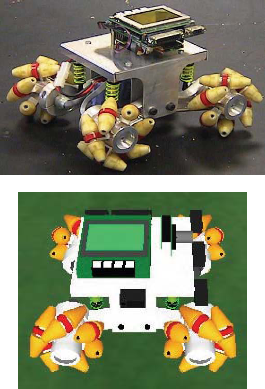
Real and simulated omni-directional robot
All sensors and actuators simulations have adjustable error models, which makes the system a valuable tool for evaluating both the functionality and the robustness of a mobile robot application.
The real robots of the EyeBot family comprise vehicles with differential steering (Figure 2), Ackermann steering, and omni-directional drives (Figure 1). The SoccerBot S4Y (Figure 2) uses two precision DC motors with encapsulated gears and encoders, three infrared distance measurement sensors (PSDs), and a digital color camera for on-board image processing. A servo is used for the ball kicker activation.

Differential drive robot SoccerBot S4Y
What all robots have in common is the EyeCon controller that allows a fast construction of a new robot system by simply plugging in DC motors, servos, and a variety of supported sensor types. The EyeCon controller is based on a 32bit Motorola M68332 microcontroller running at 25 MHz with 2MB RAM, 512KB ROM (for operating system and user programs) and has a number of standard interfaces and free I/O ports (3 serial ports, 1 parallel port, 8 digital inputs, 8 digital outputs, 16 timing I/Os, digital camera interface). A full user console is included with a graphics LCD, input buttons, speaker and microphone. SoccerBot robot and EyeCon controller are available from InroSoft, http://inrosoft.com
Software development is performed on a PC or workstation under Windows or Linux with cross compilers for C and C++ as well as for 68000 assembly language. Executables are transferred via a serial connection to the controller and can either be executed directly or stored in the controller's flash-ROM area.
The RoBIOS operating system (Bräunl, T., 2006) comprises a comprehensive list of library functions to assist with motor control, sensor feedback, multi-tasking, and user interface design for robot programs. It also comprises a monitor program to assist in downloading programs via RS232, executing and storing programs, and setting various I/O parameters.
The EyeCam camera on-board the mobile robots can take images up to a resolution of 356×292 in Bayer format, however, we usually use a much lower resolution of 60×80 pixels converted to RGB. Although many people believe this resolution to be insufficient, images in Figure 4 taken with the on-board EyeCam at 60×80 pixels reveal that this resolution is indeed sufficient for most of the typical applications with small autonomous robots. Since we have to deal with limited processing power, we rather accept a lower resolution in a trade-off with higher frame rates for image processing. Achievable frame rates are up to 15 fps (frames per second) when only reading an image and displaying it on the on-board LCD. Frame rates will drop depending on the image processing tasks performed and the number of other background tasks being performed on the controller. The camera interface to the controller is 8bit parallel with a FIFO buffer (4K×9bit) to reduce the amount of CPU interrupts required for data transfer.

EyeCon controller M5

Images taken with EyeCam, 60×80 pixels
In this Chapter, we are presenting two mobile robot applications that will give an insight into the functionality and capabilities of the EyeSim simulation system.
Maze Search
Searching a maze has been a popular robot competition task for over 20 years. In fact, the “MicroMouse Contest” was the first mobile robot competition and has run since the 1980s (Christiansen, C., 1977), (Allan, R., 1979), (Bräunl, T., 1999). A robot is let to explore a previously unknown maze, then has to return to the starting point and has several tries to reach the goal in the shortest time. This task is of particular interest because it requires a combination of algorithm design and real-world robustness. One could describe this as the extension of a Computer Science task (to design the exploration algorithm as a mathematical model - or in a perfect world) to a Computer Engineering task (to make the algorithm work robustly in the real world with all its imperfections).
The advantage of the EyeSim simulation system is that it can be used for both parts of the task. First, we can deactivate all error models. This means the robot will always drive exactly the desired distance, it will always turn exactly about the desired angle, and its sensors will always return the correct values. This simplifies the maze problem to a pure algorithm problem and the simulation system can be used to debug the program logic.
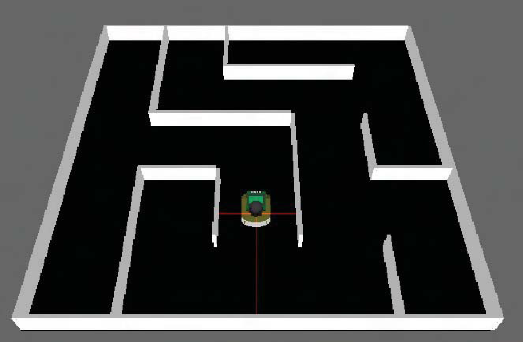
Mobile robot during maze exploration
When this stage has been achieved successfully, the program is still far from being able to succeed in driving in a real robot environment. There will always be minor errors in the robot's distance sensors, the robot will overshoot or stop short its driving command by a small amount, and it will turn a few degrees too far or too short. So the robot will slowly drift from its desired trajectory.
Therefore, the robot program has to be extended to allow for a robust or fault tolerant driving in a real maze environment. In EyeSim we can simulate this scenario by setting realistic error models for the robot's sensors and actuators, e.g. derived from measurements with a real robot. The (improved) robot application program can then be tested under these more realistic conditions. If the program masters the simulation with error settings, it will be ready to be used on a real robot.
So to start, we look at the algorithm in perfect conditions. To find the shortest path, we can implement a recursive algorithm that explores the complete maze (see Program 1). In every cell the robot senses the distance to left, front, and right, then enters the information about surrounding walls in its local data structure. This allows building a complete model of the maze structure.
For every new cell the robot enters (beginning with the start cell), it follows this recursive procedure:
If there is no wall to the left, then recursively explore cell to the left (then return to this cell) If there is no wall straight ahead, then recursively explore cell straight ahead (then return to this cell) If there is no wall to the right, then recursively explore cell to the right (then return to this cell)
Every new cell that the robot enters has to be marked in a data structure, so the robot knows which cells it has already visited. This is essential for the algorithm in order to terminate properly.

Maze exploration
Figure 6, top, shows the robot during the maze exploration, while the screen shot at the bottom left display the robot's local data structure after exploration. The robot now has a map of the maze and can use it for finding the shortest path. For example, the robot starts in the bottom left cell with [y, x] = [0, 0] and has to find the shortest path to the top right cell [4, 4] (see Figure 6, bottom right).

Maze exploration and result
We use a “flood fill” algorithm to find the shortest path from the start cell (bottom left) to any goal cell (see Figure 7). The start cell [0, 0] can be reached in zero steps by default, the neighboring cell [1,0] in 1 step. We now compute the distance from each newly reached cell to all their neighbor cells (in case there are no walls in-between). If cell [y, x] is reachable in k steps, then neighbor cells [y+1, x], [y-1, x], [y, x+1], [y, x-1] are all reachable in k+1 steps, provided there are no walls in-between and we have not already established a shorter path to any one of these in a previous step.
We continue with this iterative process until we have reached the goal cell or until we have visited all reachable cells (the goal would not be reachable in this case).
We can see the distance for goal cell [8, 8] equals 40 in Figure 7. To finally find the actual path (and not just the distance), we work our way backwards from the goal to the start cell. In every step from a cell with distance k, we choose the next cell with distance k-1, then k-2, and so on down to 0 at the start cell [0, 0]. Storing the driving direction in each step, we can now go directly from start to goal along the shortest path: straight, straight, turn|right, straight, straight, turn|right, and so on.
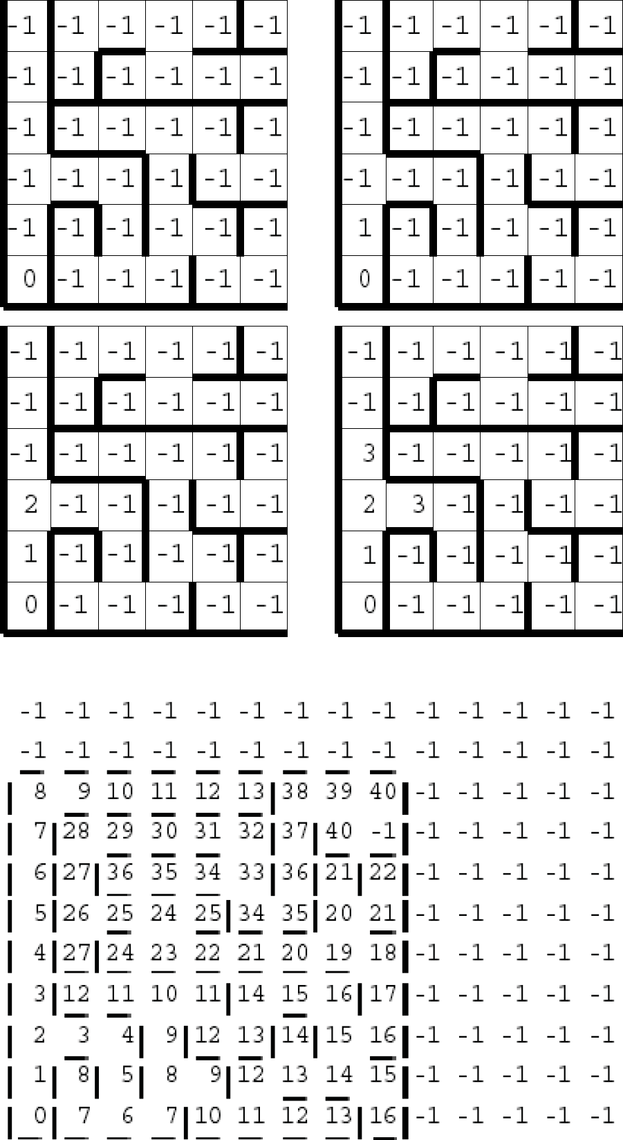
Step-wise execution of the flood-fill algorithm
The capability to produce a synthetic camera image from the robot's point of view that can be used for onboard image processing, is one of the biggest achievements of EyeSim. This virtual camera can be placed at any position and orientation relative to the robot (specified in the “robi” parameter file) and can even be mounted on simulated servos in order to perform camera pan and tilt operations. Image acquisition in simulation is handled through the same RoBIOS system calls (e.g. CAMGetColFrame) as for the real robot. Images can be displayed on the robot's LCD console (e.g. by calling LCDPutColorGraphic) and manipulated by any image processing routines.
We are presenting color object detection as a sample application. In a simple environment we have placed a red ball on one side and the robot on the other, facing away. In Program 2, we use a top-down program design strategy. We assume we have an image processing routine for ball detection (ColSearch), and then write our main program around it. In a loop, we read a camera image and display it on the LCD, then call our detection routine ColSearch, and print its results as text on the LCD (using LCDPrintf). While we are not close enough to the object (here: the detected ball diameter is less than 20 pixels), we continue driving. If the detected ball position equals −1 (no ball detected) or is between 0 and 20 (ball detected in the left image third), we rotate the robot to the left (VWDriveTurn). Is the detected ball position between 60 and 79 (ball detected in the right image third), we rotate the robot to the right, otherwise we drive a short distance forward (VWDriveStraight).
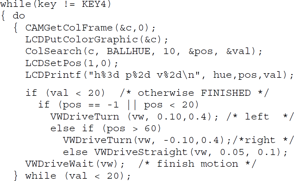
Color object search
Now we have a look at the implementation of the ball detection routine (ColSearch, see Program 3). Since color objects are easier to detect in the HSV color model (hue, saturation, value) than in the camera output format RGB (red, green, blue), we convert each pixel from RBG to HSV in the process.

Color image analysis
In a loop over all pixels, we generate a column histogram. This means we count for every column the number of pixels with a color (hue) that is similar to (matches) the desired object color (obj|hue). With this, we get a number representing the concentration of the desired color value for each column. We only have to find the maximum value over all columns in order to find the ball position. As result from function ColSearch, we return the column number (pos) with the highest concentration of matching color values (val).
Figure 8 shows the execution of the object detection program. At the beginning of the experiment the robot is facing the wall, not being able to see the ball. Following the algorithm from Program 2, the robot turns on the spot until the ball is being detected in the middle third of its local camera image. The robot then drives towards the ball and corrects its orientation in case the ball drifts towards the left or right image border.

Object detection with on-board camera
Note that this algorithm requires the ball to be visible from every board position; otherwise the robot would spin forever. An alternate solution could be to drive to various points in the environment and start searching for the ball locally.
Each robot is represented by a client, which communicates with the server through a bi-directional message channel. The server initializes the simulation, administers states of the “world” (including positions of robots and objects), synchronizes individual robots, and interacts with the fltk graphical user interface (GUI). The implemented client-server architecture does provide for a distributed simulation, i.e. each robot can in principle be simulated on a different computer system, linked via a network. In the current version, however, the simulation is started as single process, with each robot occupying one or more threads, since robots may use local multi-tasking. The server has been designed in a way such that the simulation can also run without the GUI.
Since the server and the robot application programs run in different threads, the only way for them to communicate is through the RoBIOS system calls (e.g. robot driving commands, sensor reading, or LCD output commands). For every RoBIOS function call, the server process calculates the current status of the simulated robot (e.g. the distance traveled since the last driving command) before executing the requested function
Time Model
A multi-robot simulation system is equivalent to a distributed system with individual local, unsynchronized clocks. Consequently, each robot has a local time and synchronization with the global system time (the time of the server, which serializes all requests, maintains the overall system state and handles the GUI) is performed whenever RoBIOS system calls are issued.
Especially when time delays can occur, it is essential to determine the exact simulated time of both sensor readings and driving commands. This is required in order to calculate (simulate) correct readings and positions in a continuously changing environment. EyeSim accomplishes these tasks by combining three different time models:
Each robot has its own virtual or local time. This is the time, which has elapsed in the simulated world of only this robot. E.g. a value of 10s means that the same program would have required 10s to run on a real robot of the EyeBot family. Incrementing of this virtual time is mainly achieved by executing RoBIOS functions and a look-up table with corresponding execution times, measured on a real robot for each RoBIOS function. At the end of each RoBIOS function, the virtual time of the calling robot will be incremented by the corresponding value from this table. The time a robot spends for executing other C or C++ code between two RoBIOS functions is being disregarded. The global time or simulation time is the current time of the whole simulation. It is maintained in the server and is discretized in intervals of 50ms. For synchronization purposes, all clients send their local time in regular intervals to the server and wait for a reply. If one client has already progressed to the next 50ms interval, it is being blocked to get in line with all other clients. After all clients have left the current interval, the server increments the global time, updates all positions of robots and objects, and any clients blocked in the old interval will be released. This mechanism guarantees that all robots will never get out of sync for more than 50ms. Real-time is finally the time, which has elapsed in the real world of the user since start of the simulation. Depending on the user's simulation settings for slow motion or accelerated motion, real-time is being synchronized with a correspondingly scaled version of global time. In real-time simulation mode, care is taken that global time and real-time are kept in sync (if this is possible within the limits of computing power of the host system used to run the simulation).
Further details to this topic and also the handling of multi-threaded robot application programs can be found in (Waggershauser, A., 2002), (Bräunl, T., 2006).
Drive Models
Two drive models are provided in EyeSim. A low-level interface that allows to specify individual motor wheel speeds and to read corresponding encoder feedbacks, and a high-level interface that allows direct specification of linear and angular velocity of the vehicle (vω interface).
For the low-level interface, the following drive systems can be specified: differential drive, Ackermann drive, and Mecanum-wheel based omni-directional drive. The vω interface assumes a differential drive vehicle.
All driving commands are internally mapped to three parameters: linear velocity v, angular velocity ω, and time span dt, after which the robot should be at rest again (dt can also assume an infinite value). For every new driving command, these three parameters are calculated and are being sent to the server together with the robot's current local time. The server then administers the current driving command for every robot and stores its position and orientation from the start of the driving command. This allows the calculation of each robot's position and orientation at a later point in time. Parameters v and ω are modeled as line segments and curve segments, which are being parameterized with time. This technique avoids common numerical errors, which would occur by using an iterative method for determining robot position and orientation (dead reckoning).
Collisions between robots and objects are implemented in a simplified manner, as they are handled independent of the graphics models of robots and objects. Each robot and each object is modeled as a 2D circle with a specified radius for collision purposes. During collision testing, all circles are tested for intersections with each other and with all straight-line wall segments. If a collision occurs between a robot and a wall, the robot simply stops in front of the wall. If a ball or another object hits a wall, it will bounce off the wall, depending on the reflection properties specified for wall and object. Since objects are not self-propelled as robots, an object-dependent friction factor is used to slow their motion down until they come to rest.
Modeling robots as 2D circles is a significant simplification, however, it has the advantage of allowing fast collision calculations, which have to be executed for every time step. With increasing computer performance it will make sense to implement a more elaborate collision model in the future, based on the actual robot contour.
Graphics Subsystem
A simple 3D graphics engine based on fltk (Fast Light Toolkit, 2005) and OpenGL has been developed and allows fast graphics rendering. Models for several robots, passive objects (balls, boxes, etc.), and environments have been designed with Milkshape3D (Milkshape3D, 2005). Two different environment formats are supported in EyeSim:
Maze format (MicroMouse, 2005), a text format used for mazes in the MicroMouse competition World format (Konolige, K., 2001), a text format specifying wall coordinates, extended from the Saphira simulation system
After processing the parameter files for environment, robot, and object description, the scene is displayed from a standard viewpoint. The display can be changed by panning, rotating, or zooming. Although the simulation is independent of the graphics interface, visualization is a great help in debugging robot applications, robot parameter files (e.g. sensor placements) and the simulator itself. The user interface provides a number of simulation features:
Simulation control (Start/pause of simulation, setting of simulation speed, viewing position and viewing angle) Visualization settings (Driving: trail; infrared sensors: lines; camera: frustrum; wireless communication: symbols) Error settings (Error in driving and odometry, error in distance sensor readings and camera image, error in wireless communication) Sensor data (Numerical representation of all sensor values for debugging purposes)
In the same way that the RoBIOS operating system has been mirrored between the real robot and the EyeSim simulation, the real robot's EyeBot controller console (LCD and input buttons) have been implemented in the simulation system. This allows running the robot application with exactly the same source code as the real robots under the RoBIOS operating system.
Each robot type is defined by a “robi” parameter file, which specifies simulation relevant robot data including the robot's name, size, maximum speed, sensor placements (PSD), and drive system. The sensor declaration is handled similarly to the real robot's hardware description table (HDT). EyeSim (and RoBIOS for real robots) provide driving commands on two levels. High-level driving commands allow the application programmer to specify the vehicle speed directly in terms of linear speed v and rotational speed. A built-in PID controller provides velocity and position control.
A low-level interface allows the control of individual motors and input of their respective shaft encoders. E.g. for differential drive, setting the same speed for left and right motor will result in a straight forward motion, while having different (positive) wheel speeds will result in driving a forward curve. For Ackermann drive (the classic automobile drive system), the rear wheels have one common motor while both front wheels are steered by a common servo. Using the Mecanum wheel design allows a vehicle with omni-directional drive to move in all directions including sideways and turning on the spot.
Multiple robots with different programs can interact in the same environment (Figure 9). Each robot has its own console window and its own settings, while the main simulation window is shared. Robots in a multi-robot application can be of different type (different robot definition and graphics files) and run different programs. Each robot's main program is run as a thread in multi-tasking mode, while each robot may contain several threads for parallel processing within a robot program.

Multi-robot application
The ability of a robot to complete a given task depends in many cases on its sensor equipment. Sensors enable a robot to model its environment, e.g. to determine its position in a maze. Robots from the EyeBot family are equipped with a color camera, PSD sensors (infra-red distance sensors), compass, inclinometers, gyroscopes, and shaft encoders. In order to provide a simulation as close to a real robot as possible, we need to implement the real sensor properties as close as possible in the simulation.
One of the most prominent features of EyeSim is the capability to simulate the on-board cameras of the EyeBot robots. This allows to perform real-time image processing on the simulated robots, e.g. for obstacle avoidance or target detection and tracking. The camera implementation in the simulator uses an offline buffer to draw the scene from a robot camera's point of view. This buffer can then be read from a robot user program with the RoBIOS system function CAMGetColFrame for color images or CAMGetFrame for grayscale images. The standard camera functions have a resolution of 60×80 pixels (extended to higher resolutions) at 24bit color per pixel.
The PSD sensors used in the real EyeBot robots comprise an infrared transmitter and an infrared receiver to measure the distance to the nearest obstacle. The raw data value of the PSD sensor depends on the position of the reflected infrared beam. Because of their relatively low cost and size, it is possible to equip a robot with multiple PSD sensors. Further advantages of this sensor type are reliability and robustness, which result from its simple construction. A look-up table is used to transform raw data values to actual distance values.
Modeling PSD sensors in the simulation is rather straightforward. A beam of a certain maximum length is cast in the direction of the sensor, where maximum sensor distance and sensor direction and position are specified in the robot description file. If the beam intersects with an object, e.g. another robot or a wall, the distance to the robot is calculated and buffered. Similar to the camera functions, a RoBIOS system call is used to read these values. Function PSDStart is used to start individual or continuous measurements and function PSDGet returns the measured distance in millimeters.
In the simulation environment, calculated sensor values are more precise than an actual measurement would be. On a real robot, there are several origins of sensor noise, drive inaccuracy, and occasional transmission errors are packet losses for the wireless communication.

Original screen image, with added salt…pepper noise, 100s…1000s noise, white Gaussian noise
In order to provide a simulation system that produces results as realistic as possible, we implemented artificial sensor errors and noise. Algorithms that have only been tested under perfect, synthetic conditions are still likely to fail in a real environment. The Gaussian noise used in EyeSim is a simplification of noise encountered in real environments, but is a significant help in the development of robust and fault-tolerant algorithms.
For PSD distance sensors and shaft encoders we implemented Gaussian noise, which results in a normal-distributed aberration from the correct sensor value. For the wireless transmission, we implemented random transmission errors and packet losses; and for the image acquisition, we implemented white noise and impulse noise, which in a real image sensor can be caused by sensor or transmission errors:
“Salt and pepper” noise (Random black and white pixels) “100s and 1000s” noise (Random color pixels) Gaussian white noise
We have presented the EyeSim simulation system that allows the simulation of multi-robot scenarios for driving mobile robots. A number of different drive systems and sensors, including a virtual color camera, are modeled and can be subjected to various realistic error models. Running a simulation without any errors helps in debugging the algorithm, while running a simulation with progressively larger amounts of error allows improving the robustness of an application.
The complete EyeSim robot simulation system and the real robot operating system RoBIOS can be downloaded for Windows or Linux from: http://robotics.ee.uwa.edu.au/eyebot/ftp/