Sage Journals: Discover world-class research

Abstract

As more engineering operations become automatic, the need for robustness towards faults increases. Hence, a fault tolerant control (FTC) scheme is a valuable asset. This paper presents a robust sensor fault FTC scheme implemented on a flexible arm manipulator, which has many applications in automation. Sensor faults affect the system's performance in the closed loop when the faulty sensor readings are used to generate the control input. In this paper, the non-faulty sensors are used to reconstruct the faults on the potentially faulty sensors. The reconstruction is subtracted from the faulty sensors to form a compensated ‘virtual sensor’ and this signal (instead of the normally used faulty sensor output) is then used to generate the control input. A design method is also presented in which the FTC scheme is made insensitive to any system uncertainties. Two fault conditions are tested; total failure and incipient faults. Then the scheme robustness is tested by implementing the flexible joint's FTC scheme on a flexible link, which has different parameters. Excellent results have been obtained for both cases (joint and link); the FTC scheme caused the system performance is almost identical to the fault-free scenario, whilst providing an indication that a fault is present, even for simultaneous faults.

Keywords

flexible arm fault tolerance robustness

1. Introduction

Fault tolerant control (FTC) is a really valuable asset for any system, and perhaps even an essential one. Even if there is a scheme to detect the fault, it might not be feasible to intervene and rectify the problem immediately, due to the nature of operation, and this could result in losses. As such, an FTC scheme can help to reduce the effect of the fault while waiting for the problem to be rectified. The objective of an FTC scheme is to minimize the degradation in performance of a system when a fault occurs. A reliable FTC scheme may help improve efficiency, productivity, reliability, generate financial savings or prevent catastrophic consequences such environmental pollution, or economic losses.

This paper is concerned with the application of an FTC scheme on a flexible joint and flexible link system, which can be a single DOF robotic manipulator. When a robotic manipulator is handling hazardous material or performing a dangerous task, a good FTC scheme is essential. There has been a lot of work done in the area of FTC applied to robotic manipulators. Kotosaka et.al. (Kotosaka, S. et.al., 1993) presented a FTC scheme for a manipulator which replans the trajectory in the event of an actuator fault, assuming that the actuator no longer functions. In the case of sensor faults however, there is no corrective action taken; as long as the system can still function within prescribed specifications. Goel et.al. (Goel, M. et.al., 2003) presented a method that minimizes the peak error of the end-effector velocity in the event of a fault. This was done by minimizing a performance index associated with the Jacobian of the faulty system. Lewis & Maciejewski (Lewis, C.L. & Maciejewski, A.A., 1997) proposed an FTC method for a multi-link manipulator subjected to locked joint failures. They determined the necessary constraints to subject each joint to, such that in the event of one of the joints failing (locking), the manipulator is still able to reach certain critical points. Ting et.al. (Ting, Y. et.al., 1994) proposed sliding mode and parameter adaptation control laws to reduce the errors caused by a fault. On the end, Shin et.al. (Shin, J.H. et.al. 1999) and English & Maciejewski (English, J.D. & Maciejewski, A.A. 1998) considered an FTC scheme for manipulators subjected to free-swinging joints that have lost torque and power. In (Shin, J.H. et.al. 1999), the authors firstly detected the faulty joint, and then controlled the system as an underactuated manipulator. In (English, J.D. & Maciejewski, A.A. 1998), the authors measured a cost function based on each joint's kinematic and dynamic parameters, and then minimized that function to make it as robust as possible to faults.

Izumikawa et.al. (Izumikawa, Y. et.al., 2002) presented a flexible joint FTC scheme for sensor faults; when a certain sensor fails, the feedback control scheme changes gains in order to not let the system performance degrade too much. In a more recent paper, Izumikawa et. al. (Izumikawa, Y. et.al., 2004) implemented an observer-based FTC scheme; when a sensor fails, the controller switches, and uses the observer's outputs instead of the original system's (faulty) outputs. Similar to (Izumikawa, Y. et.al., 2002, Izumikawa, Y. et.al., 2004), the application in this paper is concerned with FTC for sensor faults. Sensor faults are faults that occur in the sensors/transducers that measure the system variables, and do not directly affect the process dynamics (in the open loop). The source of these faults could be wear and tear of the sensor, prolonged use without calibration, or a total failure of the sensor. In the closed loop, these faults will affect the process if the sensor measurements are used to generate the input control signal. Therefore, the faults will cause degradation in the system performance. The FTC scheme consists mainly of a fault reconstruction scheme (Tan, C.P. & Habib, M.K. 2004) where the outputs are firstly separated into non-faulty and potentially faulty components. The control input and non-faulty outputs are fed into a linear observer (Tuenberger, D.G., 1971) to generate an estimate of the states. A reconstruction of the sensor fault is obtained by subtracting a function of the estimated states from the measured outputs, and the result is multiplied by a scaling matrix. The reconstruction is subtracted from the faulty sensor to get a ‘irtual sensor’. In an ideal situation when the fault is estimated perfectly, the virtual sensor should be give the output's correct reading. The virtual sensor (instead of the normally used faulty output) will then be used to generate the control signal, and the degradation in system performance should be eliminated. However, in a real system, there are system non-linearities and uncertainties, which cannot be fully modelled. These elements will make the state estimate inaccurate, which in turn will corrupt the fault reconstruction as well as the output of the virtual sensor. Therefore, in this paper, a design method is presented to minimize the effect of the non-linearities/uncertainties on the virtual sensor, using the Bounded Real Lemma (Peterson, LR. et.al. 1991). This paper is organized as follows; firstly the FTC scheme and its design method are presented. Then descriptions of the flexible joint and flexible link are given. Following that, test results for the flexible joint are presented, where the sensors are subjected to 2 fault extremes: total failures (where the sensor gives a zero reading) and incipient faults (where the sensor drifts very slowly and unnoticeably). Then the FTC scheme for the flexible joint is tested for robustness by implementing it on a flexible link. Finally conclusions are made. The results obtained are very good, whereby the FTC scheme provides a very accurate reconstruction of the fault (which then indicates that a fault is present), and improves the system's faulty performance such that it is very close to the fault-free scenario. Furthermore, the FTC scheme implemented on the flexible link shows very good results too, which demonstrates the robustness of the scheme. Also, this method proved successful in handling simultaneous faults. This proves the effectiveness of this approach. In this paper, all signal vectors are assumed to be functions of time t.

2. The robust fault tolerant control scheme

Consider the system modeled by the state-space equations below

\begin{array}{l} \frac{d x}{d t} = A x + B u + Q ξ \\ y = C x + F f \end{array}

(1)

where x ∈ ℝⁿ are the states, y ∈ ℝ^p are the measured outputs, u ∈ ℝ^m are the control inputs, and f ∈ ℝ^q are faults that could possibly act on the sensors. If the output y is used to generate the control signal u in the feedback loop then the performance of the system will be degraded, because y is faulty. Assume also that rank(C) = p, rank(F) = q,p ≥ q. This means that some sensors are not fault prone, which is reasonable as some have very high reliability (Tan, C.P. & Edwards, C., 2003) This can be realized by applying hardware redundancy on those sensors. The vector ζ ∈ ℝ^k encapsulates the uncertainty present in the system, such as nonlinearities or unmodelled dynamics (Chen, J. & Patton, R.J., 1999).

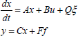
Let T_r ∈ ℝ^p×p be an orthogonal matrix such that

T_{r} F = [\begin{matrix} 0 \\ F_{2} \end{matrix}]

(2)

where F₂ ∈ ℝ^q×q is nonsingular. The matrix T_r can be computed by a simple QR decomposition on F . Scaling the output y by T_r, and then partitioning appropriately yields

T_{r} y = {\begin{cases} T_{r, 1} y = y_{1} = C_{1} x \\ T_{r, 2} y = y_{2} = C_{2} x + F_{2} f \end{cases}

(3)

where y₁ ∈ ℝ^p-q and T_r,1,T_r,2, C₁, C₂ are appropriate partitions of T_rC. The output vector has now been effectively partitioned into nonfaulty (y₁) and faulty (y₂) components. Notice now that the subsystem (1) and y₁ in (3) make up a fault-free state-space system.

Assume further that (A, C₁) is detectable, and consider an observer (Luenberger, D.G., 1971) for the fault-free system (1) and (3)

\frac{d x_{e}}{d t} = (A - L C_{1}) x_{e} + B u + L y_{1}

(4)

where x_e ∈ ℝⁿ is an estimate for the state x and L ∈ ℝ^n×(p-q) is a design matrix such that A - LC₁ is stable. Define e:= × – x_e as the state estimation error, and combine (1), (3) and (4) to get

\frac{d e}{d t} = (A - L C_{1}) e + Q ξ

(5)

Define a (measurable) reconstruction for the fault f as

f_{e} = W T_{r} (y - C x_{e}), W = [W_{1} F_{2}^{- 1}]

(6)

where W₁ ∈ ℝ^q×(p-q) is an arbitrary design matrix. Suppose the fault reconstruction in (6) is used to make a virtual sensor in the following way (Edwards, C. & Tan, C.P., 2006)

y_{o} = y - F f_{e}

(7)

where y_o will be used to generate the control signal u in the feedback loop. Define z:= y_o - Cx to be the difference between the virtual sensor y_o and the fault-free output Cx . From equations (6) and (7), as well as the definition of the error e, it follows that

z = - F W T_{r} C e

(8)

If a good fault reconstruction can be obtained (f_e ≈ f) then the virtual sensor y_o in (7) will be very close to the fault-free output Cx, resulting in z being small. Then, if the feedback control scheme uses y_o instead of y, then the performance of the system will not be badly affected though a fault is present. Hence, the objective is to minimize z.

Equations (5) and (8) show that ζ is the excitation signal of z . According to the Bounded Real Lemma (Peterson, I.R., et.al. 1991), if there exists a solution to P,Y,W₁, γ that satisfies the following inequalities

[\begin{matrix} X_{1} + X_{1}^{T} & P Q & (F W T_{r} C)^{T} \\ Q^{T} P & - γ I_{k} & 0 \\ F W T_{r} C & 0 & - γ I_{p} \end{matrix}] < 0

(9)

P = P^{T} > 0

(10)

where X₁ = PA-YC₁, then the H_∞ norm from ζ to z will not exceed the positive scalar γ. Hence it makes sense to minimize z . This problem can be easily solved using the Linear Matrix Inequalities (LMI) Control Toolbox (Gahinet, P., et.al. 1995), which will return values for P,γ,W₁,Y . The gain L can then be calculated as L = P⁻¹ Y .

A schematic diagram of the FTC scheme is shown in Figure 1.

Fig. 1.

Schematic diagram of the fault reconstruction scheme used in this paper. The signals r indicates the reference value for the output y. The block H(s) denotes the controller, and G(s) denotes the system as in (1) – (2).

2.1. Feasibility of the scheme

From control theory and the observer in (4), the condition for this method to be feasible is that any there must be a matrix L such that A –LC₁ is stable. This would therefore require the pair (A,C₁) to be detectable (Luenberger, D.G. 1971). Therefore, if the system is open loop stable, then the method in this paper is feasible for all possible sensor faults. If A has unstable eigenvalues, then the feasibility will depend on C and F . The greater the number of faults q, the rank of F will increase, and the chances of feasibility of this method will decrease. If all sensors are faulty p = q, then C₁ does not exist, and it would render this method infeasible for unstable systems.

If (A,C₁) is not detectable, the number of faulty sensors q need to be reduced, by making some of them ‘unfaulty’. This can be done by applying hardware redundancy to those sensors, and some voting system can be used for their fault tolerance. This of course is not ideal as hardware redundancy adds to weight and space. The limitation of this paper is shown here. However, it is an improvement as it reduces hardware redundancy.

3. The flexible manipulator systems

The system consists of a rigid arm mounted on a body, which is in turn mounted to a DC motor by two thumbscrews. Two springs attach the arm to the body, thus resulting in a flexible joint. A picture of the flexible arm is shown in Fig. 2.

Fig. 2.

A picture of the flexible arm system. In the foreground is the flexible arm. On the right of the picture is the computer and on the left of the picture is the power supply and interface system.

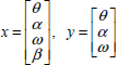
There are three measured outputs: the angle of the DC motor θ (rads) (measured by an encoder), the angular velocity of the motor ω (rad/s) (measured by a tachometer), and the deflection of the rigid arm relative to the body α(rad) (measured by an encoder). The control input to the system is the motor voltage V_m (volts). The system is interfaced to Matlab and Simulink via the Real Time Workshop Toolbox. Hence, the controller and FTC scheme are implemented using Simulink. In order to get the linear model in the notation of (1) – (2), the system was linearized about the point α = 0.

Define the states and outputs respectively as

x = [\begin{matrix} θ \\ α \\ ω \\ β \end{matrix}], y = [\begin{matrix} θ \\ α \\ ω \end{matrix}]

From the equipment data sheet and the definition of states and input, the matrices A and B respectively in the notation of (1) – (2) are

A = [\begin{matrix} 0 & 0 & 1 & 0 \\ 0 & 0 & 0 & 1 \\ 0 & 483.1 & - 28.3 & 0 \\ 0 & - 837.2 & 28.3 & 0 \end{matrix}], B = [\begin{matrix} 0 \\ 0 \\ 49.7 \\ - 49.7 \end{matrix}]

(11)

From the definition of the outputs, the output distribution matrix is C = [I₃ 0]. A controller was implemented to make θ follow a reference θ_d and also to minimize arm oscillation α. Denote the tracking error for the arm angle θ as

\tilde{θ} = θ_{d} - θ

Then the controller was such that the control input V_m had the following structure

V_{m} = 14.77 \tilde{θ} - 27.23 α + 1.90 ω + \frac{0.66 s}{0.004 s + 1} α

(12)

The flexible link system is very similar to the flexible joint, except that it has a flexible link instead of rigid arm, hence requiring no springs. The control input and first two outputs are the same as for the flexible joint. The third output is the link deflection α (cm) measured by a pair of strain gauges. In the same way as before, the system was linearized about α = 0 and it resulted in a similarly structured model (with the same definition of states and control input) of

A = [\begin{matrix} 0 & 0 & 1 & 0 \\ 0 & 0 & 0 & 1 \\ 0 & 489.2 & - 32.0 & 0 \\ 0 & - 844.5 & 32.0 & 0 \end{matrix}], B = [\begin{matrix} 0 \\ 0 \\ 56.2 \\ - 56.2 \end{matrix}]

(13)

A similar controller was implemented for the same purpose as before, such that

V_{m} = 20 \tilde{θ} - 93.81 α + 3.38 ω + \frac{26.56 s}{s + 30} α

(14)

4. Design and implementation of FTC scheme

It was assumed that the α and ω sensors are fault-prone. The θ sensor has to be assumed perfect, because it was found that a fault in the that sensor would cause (A,C₁) to have an unobservable mode at 0, which is marginally unstable, hence undesired. Due to the linearization process, any nonlinearities will be in rows 3–4 of the matrices (A,B). In addition, the discrepancies (parameter deviations) between the flexible joint and flexible link are also all in rows 3–4. Notice that there are no discrepancies in rows 1–2 because it is simply a mathematical truth. Hence a suitable choice of F and Q (in the notation of (1) – (2) is

F = [\begin{matrix} 0 \\ I_{2} \end{matrix}], Q = [\begin{matrix} 0 \\ I_{2} \end{matrix}]

For this choice of F, it was found that (A,C₁) had no unobservable modes, and hence this method is feasible for this system.

In synthesizing the FTC scheme, several additional inequalities were added to (9) to ensure that the poles of the FTC scheme (the eigenvalues of A – LC₁) to lie in a pre-specified region in the complex plane, specifically, in the intersection of two regions; the first region is a conic sector centred at the origin with an internal angle of 2θ, symmetric about the real axis. This is to ensure that the FTC scheme has a damping ratio of at least ζ = cos θ. The second region is vertical strip between a and b on the real axis where a < b . The bound b is to guarantee fast convergence, and a is to ensure that the eigenvalues of A – LC₁ are not too far in the LHP resulting in a very large and numericaly ill-conditioned value of L. From (Gutman, S. & Jury, E. 1981), the following inequalities will force the eigenvalues of A – LC₁ to lie in the specified regions

[\begin{matrix} (X_{1} + X_{1}^{T}) \cos θ & (X_{1} - X_{1}^{T}) \sin θ \\ (- X_{1} + X_{1}^{T}) \sin θ & (X_{1} - X_{1}^{T}) \cos θ \end{matrix}] < 0

(15)

X_{1} + X_{1}^{T} - 2 b P < 0

(16)

- X_{1} - X_{1}^{T} + 2 a P < 0

(17)

Choosing θ = 45° to ensure $ζ = \frac{1}{\sqrt{2}}$ , as well as a = −100, b = −2, and minimizing γ subject to (9), (10), (15), (16) and (17) yielded

L = 10^{4} \times [\begin{matrix} - 0.0219 \\ - 0.1881 \\ - 2.1045 \\ 0.4239 \end{matrix}], W_{1} = [- 32.4651 - 148.2482]

and γ = 0.0135 (which is small) and A - LC₁ has eigenvalues at {–97.71 ± j84.83, −27.02 ± j18.52} (within the bounds). The small value of γ indicates that the FTC scheme is robust, and does not necessarily require the disturbance ζ to be small.

Without any of the bounds mentioned above (inequalities (15) – (17) not implemented), the eigenvalues of A – LC₁ are unconstrained, becoming very large in magnitude. This caused L to have an unreasonably large value (in the order of 10¹²), and be numerically ill-conditioned, and possibly affect the results.

In the tests that follow, for the faulty outputs α, ω, denote α_t, ω_t as true outputs and α_m, ω_m as measured (sensor) outputs. If the faults in the sensors are denoted as α_f, ω_f, then α_m = α_t + α_f and ω_m = ω_t + ω_f. In reality, the true outputs are not measurable. However, the system is interfaced to Simulink and the faults are induced there at signal level, making the true outputs measurable. This is to aid illustration.

4.1 Test results: Total failures

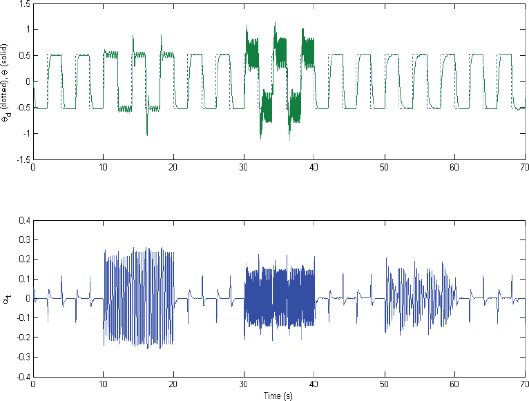
In the first test, for the flexible joint, the system was run free of fault, and the result in shown in Fig. 3, where θ follows θ_d and α_t is at a reasonably small value. Then, failures were induced. During the time range 10s < t < 20s, both the sensors for α,ω failed α_m = ω_m = 0. Then, at 30s < t < 40s, the ω sensor failed and at 50s < t < 60s, the α sensor failed. This is shown in Fig. 4. It is clear that θ has been very adversely affected when the ω sensor failed, but not significantly affected when the α sensor failed. As for α_t, it is obviously adversely affected in all faulty conditions. During the test, when the ω sensor failed, it was visually observed that the whole system was vibrating very violently, which is a very hazardous situation in practice. The results show how sensor faults affect the system's performance in the closed loop.

Fig. 3.

Flexible joint, fault free scenario

Fig. 4.

Flexible joint, with failures

Following that, the FTC scheme was put in place (u generated from y_o instead of y), and the same scenario was repeated. Fig. 5 shows θ and α_t. Compared with Fig. 4, it is clear that the FTC scheme improves the performance and restores it very closely to the fault-free scenario. This situation of total failure can be indicated by observing the sensor readings α_m,θ_m which are zero during the failures. Hence, from the results, the FTC scheme restores the performance very closely to the fault-free scenario and does not degrade system performance even when there are no faults. It can also indicate that the sensor is faulty (through the reconstructions and measured outputs), even though performance is very close to the fault-free case, so that corrective action can be taken. Finally, it is able to also handle the case of simultaneous faults without any additional degradation. A further test was conducted, where the arm was set to move in a bigger range, to show that the FTC scheme is not constrained only to a small region from the starting point. The arm angle θ was set to move to 90° clockwise and anti-clockwise in steps of 30° (staircase pattern) every 3 seconds. This corresponds to a total range of 180°. Then, at 5s < t < 10s, both the sensors for α, ω failed, and at 15s < t < 20s and 25s < t < 30s, the ω and α sensors respectively failed. Fig. 6 shows θ and α_t which have been severely degraded when the failures occur. Then the FTC scheme was put in place and Fig. 7 shows the corresponding response. It is clear that the performance has been restored very closely to the fault-free scenario. Therefore, the FTC scheme proposed in this paper is valid not only for a small neighbourhood around the starting point, but also for a large range of movement.

Fig. 5.

Flexible joint, with failures and the FTC scheme put in place

Fig. 6.

Flexible joint moving in a larger range, with failures

Fig. 7.

Flexible joint moving in a larger range, with failures and the FTC scheme put in place.

Now, the FTC scheme (designed for the flexible joint) is tested for its robustness by implementing it on the flexible link with its controller (14). Again it was firstly run fault-free, and Fig. 8 shows the responses of θ α_t. Then, the fault scenario as for the flexible joint was simulated. Fig. 9 shows θ and α_t. As before, during the sensor failures the system's performance is adversely affected. Then the FTC scheme is put in place with the same failures. Fig. 10 shows θ and α_t which have been restored to the fault-free condition. It is clear that the FTC scheme does not degrade system performance in the fault-free scenario. Hence, as in the case of the flexible joint, this FTC scheme (designed based on the flexible joint) has produced the same results for the flexible link, proving its robustness.

Fig. 8.

Flexible link, fault free scenario

Fig. 9.

Flexible link, with failures

Fig. 10.

Flexible link, with failures and the FTC scheme put in place

4.2 Test results: Incipient faults

The strength of this FTC scheme is that it can also handle slowly varying incipient faults, because of its ability to reconstruct the fault. Incipient faults are difficult to detect and could prove catastrophic if left undetected for long periods of time. Both the sensors of ω and α were subjected incipient faults during the time 10s < t < 90s. Then at 110s < t < 190s the ω sensor is faulty, and then at 210s < t < 290s the α sensor is faulty.

Fig. 11 shows the response of θ, ω_t and α_t. It can be seen that θ experiences a drift, which is expected due to the incipient faults in other sensors. Because the faults are incipient, their effects are not obvious on the measured values. However, these faults could grow over a period of time and have adverse consequences. Then the FTC scheme was put in place, and Fig. 12 shows that θ now tracks θ_d very closely. The responses for ω_t and α_t show no significant difference as before. Fig. 13 shows the reconstructions of ω_f, α_f which indicate that there are incipient faults occurring. Hence, the reconstruction signals can be used to indicate the presence of faults and corrective action can be taken.

Fig. 11.

Flexible joint, with incipient faults on the sensors

Fig 12.

Flexible joint, with incipient faults and the FTC scheme put in place

Fig. 13.

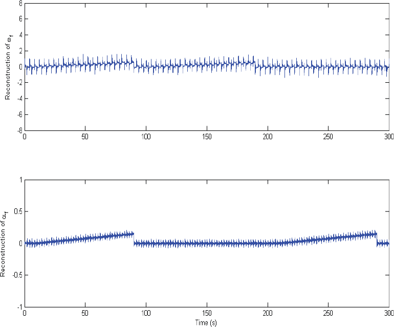
Flexible joint, the reconstructions of the incipient faults

5. Conclusion

The results in this paper show how sensor faults (especially total failures) can degrade the performance of a system and perhaps even cause catastrophes and accidents. However, more importantly, it shows how an FTC scheme restores the system performance very closely to the fault-free scenario (preventing all the above mentioned adverse situations), while indicating (through the reconstruction) that a fault is present. In addition, the robustness was demonstrated by implementing the scheme (designed for the flexible joint) on the flexible link. The results also showed the effectiveness of the scheme in dealing with simultaneous and incipient faults.

References

Chen

& Patton

R.J.

(1999). Robust model-based fault diagnosis for dynamic systems. Kluwer Academic Publishers.

Edwards

& Tan

C.P.

(2006). Fault tolerant control using sliding mode observers. Control Engineering Practice, pp vol. 14, 897–908.

English

J.D.

& Maciejewski

A.A.

(1998). Fault tolerance for kinematically redundant manipulators: anticipating free-swinging joint failures. IEEE Transactions on Robotics and Automation, vol. 14, pp 566–575.

Gahinet

Nemirovski

Laub

A.J.

& Chilai

(1995). LMI Control Toolbox, Users Guide, The MathWorks Inc.

Goel

Maciejewski

A.A.

Balakrishnan

& Proctor

R.W.

(2003). Failure tolerant teleoperation of a kinematically redundant manipulator: an experimental study. IEEE Transactions on Systems, Man and Cybernetics – Part A: Systems and Humans, vol. 33, pp 758–765.

Gutman

& Jury

(1981). A general theory for matrix-root clustering in subregions of the complex plane. IEEE Transactions on Automatic Control, vol. 26, pp 853–863.

Izumikawa

Yubai

& Hiraj

(2004). Fault tolerant control system of flexible arm for sensor fault using reaction force observer. IEEE International Workshop on Advanced Motion Control, Kawasaki, Japan, pp 583–588.

Izumikawa

Yubai

& Hori

(2002). Vibration suppression control of flexible arm robot by PD gain switching considering sensor failure. IEEE International Conference on Industrial Technology, Bangkok, Thailand, pp 684–689.

Kotosaka

Asama

Kaetsu

Endo

Sato

& Nakayama

(1993). Fault tolerance of a functionally adaptive and robust manipulator. IEEE International Conference on Intelligent Robots and Systems, Yokohama, Japan, pp 294–300.

10.

Lewis

C.L.

& Maciejewski

A.A.

(1997). Fault tolerant operation of kinematically redundant manipulators for locked joitn failures. IEEE Transactions on Robotics and Automation, vol. 13, pp 622–629.

11.

Luenberger

D.G.

(1971). An introduction to observers. IEEE Transactions on Automatic Control, vol. 16, pp. 596–602.

12.

Peterson

I.R.

Anderson

B.D.O.

, & Jonckheere

E.A.

(1991). A first principles solution to the nonsingular H_∞ control problem. International Journal of Robust and Nonlinear Control, vol. 1, pp 171–185.

13.

Shin

J.H.

Lee

L.Y.

, & Lee

J.J.

(1999). Robust fault tolerant control framework for robot manipulators with free-swinging joint failures: Fault detection, identification and accomodation. IEEE International Conference on Intelligent Robots and Systems, pp 185–190.

14.

Tan

C.P.

& Edwards

(2003). Sliding mode observers for robust detection and reconstruction of actuator and sensor faults. International Journal of Robust and Nonlinear Control, vol. 13, pp 443–463.

15.

Tan

C.P.

& Habib

M.K.

(2004). Implementation of a sensor fault reconstruction scheme on an inverted pendulum. Asian Control Conference, Melbourne, Australia, pp 1433–1438.

16.

Ting

Tosunoglu

& Fernandez

Control algorithms for fault tolerant robots. IEEE International Conference on Robotics and Automation, pp 910–915.

Tolerance Towards Sensor Faults: An Application to a Flexible Arm Manipulator

Abstract

Keywords

1. Introduction

2. The robust fault tolerant control scheme

3. The flexible manipulator systems

References