Sage Journals: Discover world-class research

Abstract

In our ongoing project on the autonomous guidance of Micro-Air Vehicles (MAVs) in confined indoor and outdoor environments, we have developed a bio-inspired optic flow based autopilot enabling a hovercraft to travel safely, and avoid the walls of a corridor. The hovercraft is an air vehicle endowed with natural roll and pitch stabilization characteristics, in which planar flight control can be developed conveniently. It travels at a constant ground height (∼2mm) and senses the environment by means of two lateral eyes that measure the right and left optic flows (OFs). The visuomotor feedback loop, which is called LORA(1) (Lateral Optic flow Regulation Autopilot, Mark 1), consists of a lateral OF regulator that adjusts the hovercraft's yaw velocity and keeps the lateral OF constant on one wall equal to an OF set-point. Simulations have shown that the hovercraft manages to navigate in a corridor at a “preset” groundspeed (1m/s) without requiring a supervisor to make it switch abruptly between the control-laws corresponding to behaviours such as automatic wall-following, automatic centring, and automatically reacting to an opening encountered on a wall. The passive visual sensors and the simple control system used here are suitable for use on MAVs with an avionic payload of only a few grams.

Keywords

OF (Optic Flow)Motion detection MAV (Micro-Air Vehicle)Hovercraft Urban canyon navigation Insect navigation Biorobotics Biomimetics Bionics

1. Introduction

Winged insects are able to navigate swiftly in unfamiliar environments by extracting visual information from their own motion. One of the most useful visual cues is the optic flow (OF), which is the apparent motion of the image of contrasting features projected onto the insect's retina. The OF is used by insects to avoid collisions (Wagner, H., 1982; Tammero, L.F. & Dickinson, M.H., 2002), to follow a corridor (Kirchner, W.H. & Srininasan, M.V., 1989), and to cruise and land (Srinivasan, M.V., et al., 1996), for example.

Based on the biorobotic approach developed at our laboratory over the past 20 years, several terrestrial and aerial vehicles equipped with OF sensing systems have been built (Franceschini, N., et al. 1992; Mura, F. & Franceschini, N., 1996; Viollet, S. & Franceschini, N., 1999; Netter, T. & Franceschini, N., 2002; Ruffier, F. & Franceschini, N., 2005; Viollet, S. & Franceschini, N., 2005), or simply simulated (Mura, F. & Franceschni, N., 1994; Martin, N. & Franceschini, N. 1994; Ruffier, F. 2004; Serres, J., et al. 2005; Serres, J., et al., 2006). The OF sensor used for this purpose is an angular velocity sensor originally designed in 1986 (Blanes, C., 1986; Franceschini, N., Blanes, C. & Oufar, L., 1986). The principle underlying this electro-optical image velocity sensor was based on findings obtained at our laboratory on the common housefly's Elementary Motion Detectors (EMDs) by performing electrophysiological recordings on single neurons while concomitantly applying optical microstimuli to two single photoreceptor cells within a single ommatidium (Franceschini, N., et al., 1989).

Studies in which honeybees flying through a narrow tunnel were closely observed have shown that these insects tend to maintain a trajectory which is equidistant from the two flanking walls (Kirchner, W.H. & Srinivasan, M.V., 1989). To explain this centring response, the latter authors proposed that the animal may balance the apparent speeds of the images of the walls perceived by their two eyes (Kirchner, W.H. & Srininasan, M.V., 1989). In the field of robotics, many research scientists have referred to this “optic flow balance” hypothesis when designing visually guided vehicles (Coombs, D. & Roberts, K., 1992; Duchon, A.P. & Warren, W.H., 1994; Santos-Victor, J., et al., 1995; Weber, K., et al., 1997; Dev,

A., et al., 1997; Carelli, R., et al., 2002; Argyros, A.A., et al., 2004; Hrabar, S.E., et al., 2005), and simulating flying agents (Neumann, T.R. & Bülthoff, H.H., 2001; Muratet, L., et al., 2005) and hovercraft (Humbert, J.S., et al., 2005). The “optic flow balance” hypothesis was tested in corridors and canyons. However, balancing the two lateral OFs would make these visually-guided robots rush into any opening in a wall, since openings give rise to virtually zero OF. To deal with this problem, some authors suggested switching to wall-following behaviour whenever the mean value of the two lateral OFs becomes larger than a given threshold (Weber, K., et al., 1997) or whenever one of the two lateral OFs is equal to zero (Santos-Victor, J., et al., 1995). Wall-following behaviour resulted in maintaining the lateral OF constant on one side by controlling the robot's heading, which meant that at a given speed the robot would tend to stay a “pre-specified distance” away from the wall (Santos-Victor, J., et al., 1995; Weber, K., et al., 1997; Zufferey, J.C. & Floreano, D., 2005).

In previous studies, we designed a bio-inspired OF based autopilot called OCTAVE, which enable a Micro-Air Vehicle (MAV) to avoid the ground by making it automatically rise or descend when flying over a shallow terrain (Ruffier, F. & Franceschini, N., 2003; Ruffier, F. & Franceschini, N., 2005). Unlike the OCTAVE autopilot, which was designed to control tasks such as takeoff, landing, wind reaction, and ground avoidance, the LORA(1) autopilot described here (LORA(1) stands for Lateral Optic flow Regulation Autopilot, Mark 1) deals with automatic wall collision avoidance, wall-following and centring problems by adjusting the yaw velocity of a miniature hovercraft. Like the OCTAVE autopilot, LORA(1) is based on an OF regulation principle. Here, however, the OF regulator adjusts the hovercraft's heading so as to maintain the OF measured equal to an OF set-point.

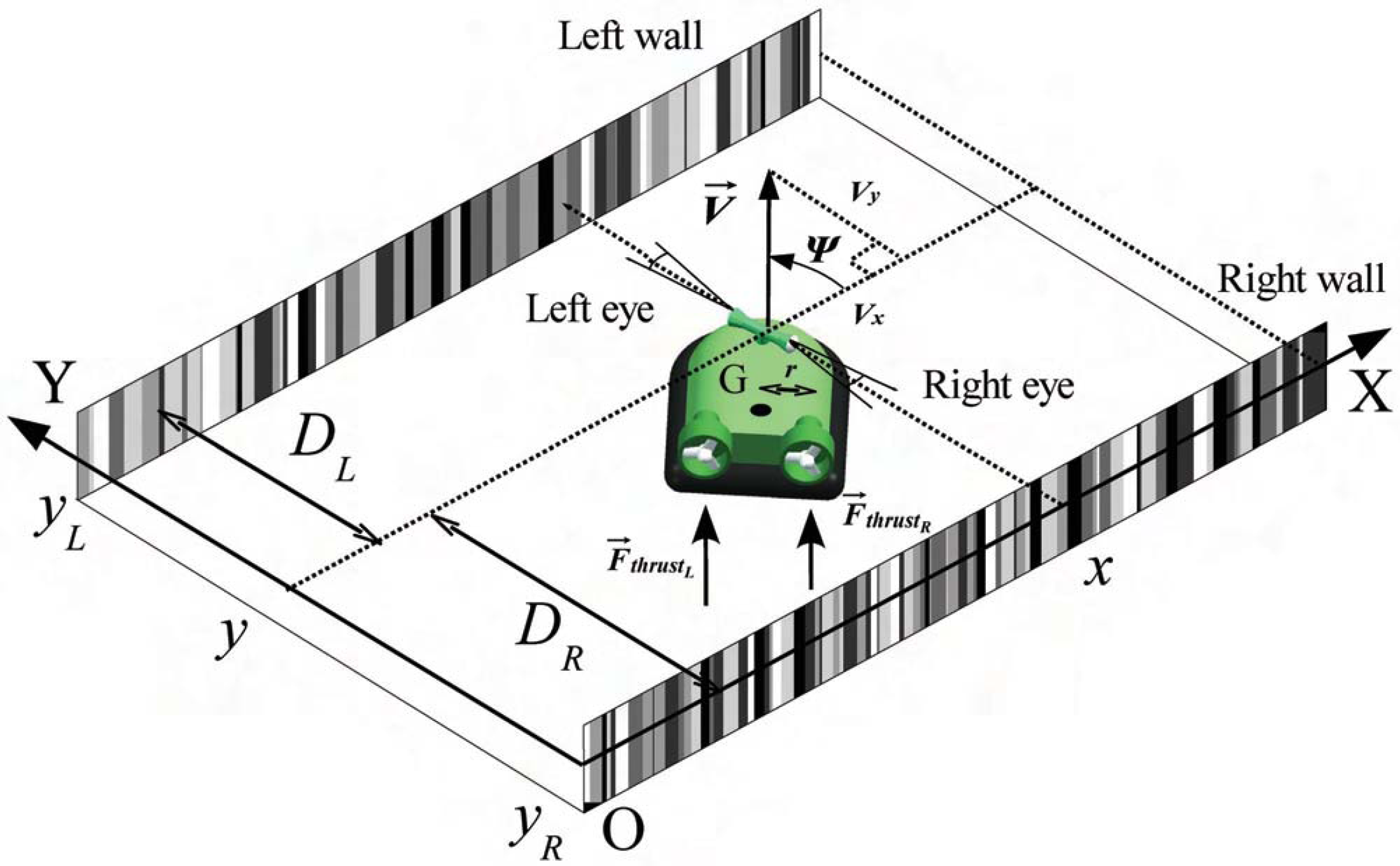
Working on a miniature hovercraft is the first step toward building an autopilot giving Micro-Air Vehicles (MAVs) lateral obstacle avoidance capacities. This type of air vehicle, which “flies” on a plane (at a ground height of ∼2mm), is endowed with natural roll and pitch stabilization characteristics. Like flying insects and air vehicles, it makes no contact with the ground while travelling and is capable of moving both forwards and sideways. Common hovercraft have three degrees of freedom: two translations along X and Y-axes, and one rotation around the Ψ-axis. They are holonomic in the plane and underactuated because they are equipped with only a pair of rear thrusters. Unlike wheeled robots, and more like insects and air vehicles, hovercraft are subjected to disturbances affecting their three degrees of freedom (such as those caused by headwind, sidewind and turbulence). Our hovercraft equipped with the LORA(1) autopilot is capable of performing various tasks such as wall-following and centring quite smoothly without having to switch abruptly from one task to another.

LORA(1) automatically adjusts the hovercraft's heading (yaw), so as to keep the robot at a “safe distance” from the walls. In this indoor study, since the hovercraft was not subjected to wind, its groundspeed was equal to its airspeed – but neither the groundspeed nor the airspeed nor the distance from the walls need to be measured in the present control system.

In a previous simulation study, we described how LORA(1) was designed to control a hovercraft where the yaw dynamics was simply a first-order low-pass filter with a time constant of 0.5s (Serres, J., et al., 2005). In the present study, we extended the hovercraft's dynamic model by carrying out a system identification in yaw on the miniature RC hovercraft (using the same robotic platform as that used by Seguchi, H. & Ohtsuka, T., 2003) and by incorporating an inertial inner loop based on a miniature rate-gyro to improve the natural dynamics of the hovercraft.

In section 2, we describe the simulation set-up used to test the LORA(1) autopilot on the hovercraft. Section 3 focuses on the insect based visual guidance principle adopted and gives details of the LORA(1) autopilot scheme. Section 4 describes some simulation runs performed by a hovercraft equipped with the LORA(1) autopilot travelling along a corridor at a “pre-set” groundspeed (1m/s), without requiring a supervisor to make it switch between the following behaviours: wall-following, centring, and reacting to an aperture encountered on a wall. Depending on the OF set-point, the hovercraft will either centre while travelling along a corridor or follow one of its two walls without being dramatically disturbed by the local absence of OF on one wall of the two walls.

2. Simulation set-up

All the present experiments are computer simulations carried out on a standard PC equipped with the Matlab™/Simulink software program with a sampling frequency of 1kHz.

2.1. The dynamic hovercraft model

2.1.1 Hovercraft yaw dynamics

The hovercraft travels at a groundspeed $\vec{V}$ over a flat surface along a corridor with randomly textured walls in terms of both the spatial frequency and the contrast (Fig. 1). In the 2-D approximation used throughout this study, the hovercraft's motion is defined by dynamic equations involving the forward thrusts (F_thrustR and F_thrustL) produced by the two rear thrusters. Since the propeller time constant is much smaller than the aero-mechanical time constant when dealing with yaw, the propeller dynamics will be neglected here. The following linearized system of equations, referred to the center of gravity G is used:

J \frac{d \dot{Ψ}}{d t} + ζ_{Ψ} \dot{Ψ} = r \times (F_{T h r u s t_{R}} - F_{T h r u s t_{L}})

(Eq. 1)

Fig. 1.

Hovercraft moving at groundspeed $\vec{V}$ along a textured corridor. The two symmetric eyes detect the right OF ω_R and the left OF ω_L, as described by Eq. 6 and Eq. 7. The pair of lateral eyes is mounted on the hovercraft with one degree of freedom in the yaw direction, which enables their gazes to be constantly oriented along the Y-axis. The autopilot adjusts the two rear thrusts differentially and thus determines the hovercraft's yaw velocity dΨ/dt.

with

\dot{Ψ} \frac{d Ψ}{d t}

(Eq. 2)

where J (0.0125kg.m²: the same robotic platform as that used by Seguchi, H. & Ohtsuka, T., 2003) is the moment of inertia of the hovercraft along the Ψ-axis, and ζ_Ψ is the rotational viscous friction coefficient along the Ψ-axis, and r (0.095m) denotes the moment arm of the rear thrusters with respect to the centre of gravity G. The hovercraft is underactuated, since the groundspeed components V_x and V_y cannot be controlled independently (Eq. 3, 4). For the purposes of the simulation, the groundspeed V is assumed to be at the “pre-set” value of 1m/s.

V_{x} = V . cos (Ψ)

(Eq. 3)

V_{y} = V . sin (Ψ)

(Eq. 4)

2.1.2. Identification of the hovercaft yaw dynamics

System identification was performed on the dynamics of the miniature RC hovercraft (Taiyo Toy Ltd., Typhoon T-3: 0.36times0.21times0.14 m) by feeding the control signal U(t) (Fig. 2) with a “chirp” commanding the two DC motors differentially. This modulated sinusoidal function started at a frequency of 0.15Hz and reached a maximum frequency of 8Hz within 50 seconds. The hovercraft's yaw velocity dΨ/dt was recorded at a sampling interval of 2ms by using a miniature rate-gyro from Analog Devices (sensitivity 5mV/(°/s), bandwidth 50Hz). The pre-process step of the input signal U(t) and the output signal dΨ/dt consisted mainly in filtering the data with a 5^th order Butterwoth band-pass filter (low cut-off frequency 0.01Hz and high cut-off frequency 8Hz). The transfer function G_Ψ(s) (Eq. 5), relating the hovercraft's yaw velocity dΨ/dt (Eq. 2) to the control signal U(t) was estimated by means of the System Identification toolbox included in the Matlab™ software package. The best fit (fit factor 0.7) was obtained with a first-order low-pass filter with a time constant of 2.14s and a static gain of 6.14rad/s/V (Eq. 5).

G_{Ψ} (s) = \frac{\dot{Ψ} (s)}{U (s)} = \frac{6.14}{1 + 2.14 s}

(Eq. 5)

Fig. 2.

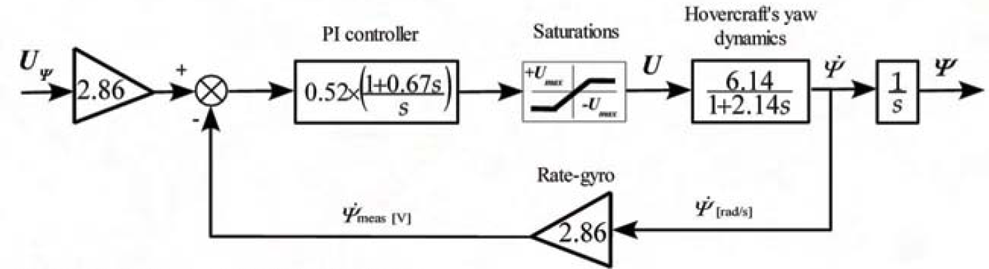
The inertial feedback loop incorporated into the LORA(1) autopilot between the variables U_Ψ and Ψ in Fig. 3 improves the hovercraft's rising time along the Ψ-axis. The hovercraft's yaw velocity $\dot{Ψ}$ is measured by means of a miniature rate-gyro (see 2.1.2) and compared with a reference input U_Ψ originating from the OF outer loop (Fig. 3). The control signal U(t) commands the differential thrust between the two rear thrusters, which determines the hovercraft's yaw velocity $\dot{Ψ}$ .

2.1.3. Yaw rate inner feedback loop

An inertial feedback loop was incorporated to improve the hovercraft's yaw dynamics (Fig. 2). The hovercraft's yaw velocity was measured by means of the miniature rate-gyro (see 2.1.2). The yaw velocity measured ${\dot{Ψ}}_{meas}$ is compared with a reference input U_Ψ, provided by the OF outer loop (Fig. 3). A proportional-integral (PI) controller was introduced into this inertial feedback loop to shorten the hovercraft's rising time and to reject any heading disturbances. The PI controller was designed by taking into account the saturations of the control signal U(t).

Fig. 3.

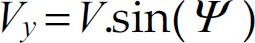
The LORA(1) autopilot (red block diagram) has one control output U_Ψ that commands the yaw angle Ψ. The groundspeed V is commanded in open loop. The Optic Flow (OF) controller C _ω (s) (Eq. 9) incorporated into the system regulates the lateral OF, which is measured by OF sensors (i.e., angular motion detectors). The output from the OF controller commands the yaw torque, on which the hovercraft's yaw velocity depends. The maximum value between the right (ω_Rmeas) and left (ω_Lmeas) lateral OFs is compared with an OF set-point ω_SET, and the direction in which wall avoidance is performed by the sign of the difference between the right and left lateral OFs measured. The wall on the right (right wall ordinate y_R) and the wall on the left (left wall ordinate y_L) are treated by the visuomotor feedback loop like disturbances (blue arrows).

2.2. Optic flow during pure translation

The hovercraft travels at a groundspeed vector $\vec{V}$ over a flat surface along a corridor with randomly textured walls in terms of both the spatial frequency and the contrast (Fig. 1). The two diametrically opposite eyes detect a right and a left OF, ω_R and ω_L, respectively (Fig. 1). The two translational OFs can be defined as follows:

ω_{R} = V_{x} / D_{R}

(Eq. 6)

ω_{L} = V_{x} / D_{L}

(Eq. 7)

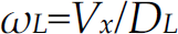
where V_x is the the hovercraft's groundspeed projected onto the X-axis, and D_R and D_L are the distances between the right and left walls, respectively. To cancel the rotational component of the OF due to the hovercraft's yaw rotation, the eyes are assumed to counter-rotate so as that they are always aligned with the Y-axis. To that aim, a micro-gyro-compass could measure the hovercraft's heading angle so as to stabilize the gaze at right angle with respect to the corridor axis (Coombs, D. & Roberts, K., 1992). The eyes therefore perform a purely translational movement and hence they detect a purely translational OF.

2.3. Eyes and optic flow sensors

Each lateral eye consists of just two photoreceptors (i.e., of two pixels), the visual axes of which are separated by an interreceptor angle Δφ = 4°. The angular sensitivity of each photoreceptor is given by a bell-shaped function where the acceptance angle (Δρ: the angular width at half height) is also Δρ = 4°. Each OF sensor is composed of the assembly of one lens/two photoreceptors driving an EMD circuit. The principle of the EMD circuit that serves as an OF sensor has been described in previous paper (Blanes, C., 1986; Franceschini, N., Blanes, C. & Oufar, L., 1986; Viollet, S. & Franceschini, N., 1999; Ruffier, F., et al., 2003). It is a nonlinear circuit where the inputs are the two photoreceptors and the output is a monotonic function of the angular velocity within a 10-fold range (from 40°/s to 400°/s) (Ruffier, F. & Franceschini, N., 2005). Whenever it does not detect any new contrasting feature, the OF sensor holds the last measured value for a period of 0.5s. The output signal from each photoreceptor is computed at each time step by summing together all the grey level patterns present in its field of view (which covers approximately three Δρ, i.e., 12°) and by weigthing the summation with a bell-shaped angular sensitivity function.

3. LORA(1) autopilot

3.1. Bio-inspiration

The visual guidance principle adopted here was inspired by findings obtained on the flight behaviour of honeybees (Kirchner, W.H. & Srinivasan, M.V., 1989). The authors of the latter study observed that honeybees tend to fly along the midline of a straight corridor (centring response), and concluded that “bees maintained equidistance by balancing the velocities of the retinal images in the two eyes” (Kirchner, W.H. & Srinivasan, M.V., 1989). Upon analyzing the flight of a tethered fruitfly, Götz noted that the yaw torque (which determines the yaw velocity dΨ/dt) results from the differential thrust of the two wings, while the forward thrust (which determines the groundspeed V) results from the total thrust of the two wings (Götz, K.G., 1968). The yaw velocity dΨ/dt and groundspeed V are the variables on which the LORA(1) autopilot guiding our hovercraft is based.

3.2 LORA(1) visuomotor feedback loop

The LORA(1) autopilot is an OF regulator (Fig. 3). The feedback signal it receives is the largest of the two OFs (left and right OFs) measured. This autopilot was designed to keep the lateral OF constantly equal to an OF set-point ω_SET. The hovercraft then reacts to any changes in the lateral OF by adjusting the yaw torque (which determines the hovercraft's yaw velocity dΨ/dt), thus leading to a change in the distance from the left (D_L) or right (D_R) wall. A sign function automatically selects the wall to be followed. For this purpose, a maximum criterion is used to select the higher OF value measured between the right OF (ω_Rmeas) and the left OF (ω_Lmeas). The OF selected value is compared with the OF set-point ω_SET (Fig. 3). In the steady state, the OF selected will therefore become equal to the set-point ω_SET. The error ε in the input to the OF controller is computed as follows:

ε = sign (ω_{Lmeas} - ω_{Rmeas}) \times (ω_{SET} - max (ω_{Lmeas}, ω_{Rmeas}))

(Eq. 8)

A lead controller Cω(s) (Eq. 9) was introduced into the visual feedback loop to improve the stability and the response stiffness.

C_{ω} (s) = 0.1 \times \frac{2.5 s + 1}{0.2 s + 1}

(Eq. 9)

The LORA(1) autopilot has two input parameters:

the OF set-point ω_SET, which defines the ratio between the forward groundspeed V_x (the groundspeed X-component) and the shorter of the two distances to the corridor walls (D_L or D_R),

the robot's groundspeed V.

4. Simulation results

4.1. Simulated visual environment

The simulated visual environment is straight a 12-metre long, 1-metre wide corridor. Its right and left walls are lined with a random pattern consisting of various grey vertical stripes covering a large spatial frequency range (from 0.069 c/° to 0.87 c/° reading from the midline) and a large contrast range (from 6% to 40%). No special steps were taken to make the two opposite patterns mirror-symmetric.

4.2. Automatic wall-following behaviour

Figure 4 shows the robot's trajectories resulting from our control scheme based on a lateral OF regulator. It can be seen from this figure that this scheme automatically generates clearance from one wall. The greater the OF set-point ω_SET, the smaller the distance to the wall will be because the latter is an inverse function of the OF set-point (Eq. 6, 7). It is noteworthy that the LORA(1) autopilot enables the hovercraft to control its distance from the wall without measuring its groundspeed or distances from the walls. In these trajectories where the two OFs measured are smaller than the OF set-point, the hovercraft can be seen to adjust its yaw velocity (which determines its groundspeed Y-component: Eq. 4), eventually generating a distance with respect to the wall (here the right one). The solid red trajectory shows the particular case where the two OFs measured (ω_Lmeas and ω_Rmeas) are equal to the set-point ω_SET. The error ε (Eq. 8) is null and the hovercraft therefore automatically follows the midline, thus adopting the behaviour known as the centring response.

Fig. 4.

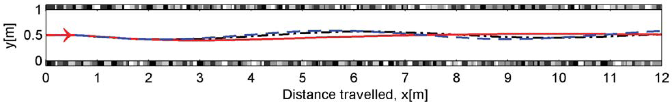
Four simulated hovercraft trajectories moving to the right (red arrow) in a one-metre wide corridor at the same groundspeed (1m/s) but with different OF set-points (solid red curve: ω_SET =115°/s; dotted curve black: ω_SET = 130°/s; dashed blue curve: ω_SET = 170°/s; dash-dotted green curve: ω_SET = 230°/s). The two walls are lined with a printed pattern showing a large spatial frequency range (from 0.069 c/° to 0.87 c/° as seen from the midline: Y=0.5m), and a large contrast range (from 6% to 40%). In these trajectories where the OF set-point is larger than either of the two OFs measured, the hovercraft adjusts its yaw torque (which determines its groundspeed Y-component: Eq. 4), and thus generates a distance to the right wall. The red central trajectory shows the particular case where the two OFs measured (ω_Lmeas and ω_Rmeas) are equal to the set-point ω_SET. In this case, the hovercraft adopts a centring response.

4.3. Automatic centring behaviour

It can be seen from Fig. 5 that when the OF set-point is never reached by the OFs measured (ω_Lmeas or ω_Rmeas), the hovercraft attempts to centre between the right and left walls, oscillating to a variable extent along the midline (Y = 0.5m). The magnitude of the oscillations depends on the error ε (Eq. 8), which cannot be cancelled by the visuomotor control loop because of the width of the corridor. The OF-field is minimum along the midline of the corridor and cannot reach a value lower than 115°/s. The error signal ε is therefore also minimum along the midline. The solid red trajectory again shows the particular case where the two OFs measured are equal to the OF set-point (ω_SET = 115°/s) and both OFs measured are close to the minimum OF-field value (red curves in Fig. 4,5). In this case, the hovercraft follows the midline without any oscillations because the visuomotor closed loop just cancels the error ε (Eq. 8).

Fig. 5.

Three simulated trajectories at the same “pre-set”groundspeed (1m/s) with an OF set-point which is never reached by two OFs measured. In all the three cases, the hovercraft can be seen to centre between the two walls, oscillating variably about the midline (blue dashed curve: ω_SET = 80°/s; black dash-dotted curve: ω_SET = 90°/s; red solid curve: ω_SET = 115°/s). The textured environment is the same as in Fig. 4.

4.4. Automatic reaction to an opening

Figure 6 shows the effect of a local absence of OF on one wall. This “no contrast” zone simulates a lack of texture or an opening. Although the hovercraft is unable to measure any OF along the 4m long aperture on its right hand side, it can be seen that it was not dramatically affected, since it just automatically followed the opposite textured wall. In the dashed black trajectory (Fig. 6), the hovercraft initially displayed centring behaviour. Along the right opening, the hovercraft came to follow the left wall and the LORA(1) autopilot generated a “safe distance” of about 0.5m from the left wall (for ω_SET = 115°/s and V=1m/s). By contrast, the dashed black trajectory shows the effect of the “no contrast” zone when the OF set-point is larger than the two measured OFs. The hovercraft followed the right wall at first and the LORA(1) autopilot generated a “safe distance” of about 0.34m (for ω_SET =170°/s and V=1m/s) with respect to this wall. The hovercraft then encountered the opening at X = 4m. The dashed black trajectory shows that from X = 4m to X = 4.5m, the hovercraft was not affected by the opening because the right OF sensor kept on measuring the right OF for another 0.5s (Fig. 6c). After this delay, the hovercraft becomes « blind » to the right wall and automatically follows the left wall, due to the change in the sign of the error signal ε (Eq. 8).

Fig. 6.

(a) Effects of a “no contrast” zone on two simulated hovercraft trajectories with the same “pre-set” groundspeed value (1m/s) but with different OF set-points (solid red curve: ω_SET = 115°/s; dashed black curve: ω_SET = 170°/s). In the solid red trajectory, the robot adopts centring behaviour and it is hardly affected by the 4-meter long “no contrast” zone along its right hand side: it automatically follows the left wall due to the change in sign of the error ε (Eq. 8). In dashed black trajectory, the hovercraft adopts a wall-following behaviour because the OF set-point (dashed black curve: ω_SET =170°/s) is larger than the minimum OF value because of the corridor width. When the hovercraft encounters to the aperture (i.e., a “no contrast” zone) on the right, it automatically turns to the opposite left wall due to the change in sign of the error ε (Eq. 8). (b) The corresponding groundspeed X-component V_x as a function of the distance travelled x. (c) Groundspeed Y-component V_y as a function of the distance travelled x.

5. Discussion and conclusion

Our present results show that the LORA(1) autopilot in which a lateral OF regulator is used to drive the yaw velocity is an efficient means of making a miniature hovercraft automatically follow a wall at a “safe distance” or centre along the midline of a corridor, while reacting appropriately to the local absence of contrast encountered on one wall. All these navigational tasks are performed with the single control scheme shown in Fig. 3 at a relatively high “pre-set” groundspeed (1m/s) compared to related works which dealt with relatively low “pre-set” groundspeed (0.08m/s in Santos-Victor, J., et al., 1995, 0.12m/s in Weber, K., et al., 1997, and 0.10m/s in Zufferey, J-C. & Floreano, D., 2005). The lateral OF regulation principle differs from the “optic flow balance” strategy derived from observations of honeybees in that it does not require a supervisor to switch between centring and wall-following behaviours, contrary to a robotic approach that consists of switching to a wall-following behaviour whenever the robot does not detect any OF on one wall (Santos-Victor, J., et al., 1995; Weber, K., et al., 1997).

The hovercraft equipped with LORA(1) exhibits a behaviour which depends on both the OF set-point ω_SET (input parameter shown in Fig. 3) and the width of the corridor. In a corridor of a given width, by increasing its ω_SET, the hovercraft will hug one wall (wall-following behaviour, Fig. 4). By decreasing its ω_SET, the hovercraft will tend to move away from the two walls thus ending up along the midline (centring behaviour, Fig. 5). However, the hovercraft attempting to centre between the walls shows variable oscillations (Fig. 5), which have two causes:

LORA(1) cannot reach the OF set-point ω_SET (see 4.3.).

A heading control system does not uncouple the lateral motion dynamics from the forward motion dynamics. The non-sliding constraint is given by differentiating Eq. 4: ${\dot{V}}_{y} = V_{x} . \dot{Ψ}$ .

The latter point also relates to the wheeled robots which roll without sliding because they are non-holonomic systems. A heading control system driving a wheeled robot shows irremediably variable oscillations for a wall-following task (Santos-Victor, J., et al., 1995; Weber, K., et al., 1997; Zufferey, J-C. & Floreano, D., 2005). By contrast, simulations of a fully actuated hovercraft equipped with a forward-plus-side-slip control system (called LORA(2) autopilot) based on two lateral OF regulators with a single OF set-point have been successfully conducted and show no oscillations in a straight or tapered corridor (Serres, J., et al., 2006). The LORA(1) autopilot we have presented here can nevertheless be applied to non-holonomic or underactuated vehicles such as rolling vehicles and aeroplanes. Implementation of the LORA(1) and LORA(2) autopilots on a miniature hovercraft (Typhoon T-3 by Taiyo Toy Ltd.) is now under way. Our study has shown that a hovercraft can navigate in a straight corridor even with a minimalistic number of pixels (only four pixels in fact) and without any metric sensors such as rangefinders or velocimeters. Combined with an OF regulator operating in the vertical plane to ensure ground obstacle avoidance (Ruffier, F. & Franceschini, N., 2003; Ruffier, F. & Franceschini, N., 2005), the LORA(1) autopilot is one more step towards developing low-cost visual guidance systems for aerial vehicle navigation in unfamiliar indoor and outdoor environments. Passive OF sensors combined with a simple processing system will be particularly suitable for use with Micro-Air Vehicles (MAVs), which impose highly stringent constraints in terms of the avionic payload and the onboard energy resources allowed.

Footnotes

6. Acknowledgements

We are grateful to M. Boyron and F. Paganucci for their expert technical assistance, to J. Blanc for her help with the English manuscript. This research was supported by CNRS (Life Science and Engineering Science) and by EU contract (IST/FET – 1999-29043).

Abbrevations

References

Argyros

A.A.

Tsakiris

D.P.

& Groyer

(2004). “Biomimetic centering behavior for mobile robots with panoramic sensors”. IEEE Robotics and Automation Magazine, Eds. Daniilides

and Papanikolopoulos

, vol. 11, Issue 4, pp. 21–30, (Dec.).

Blanes

(1986). “Appareil visuel élémentaire pour la navigation à vue d'un robot mobile autonome”. M.S. Thesis in Neurosciences (“DEA” in French), Neurosciences, Univ. Aix-Marseille II.

Carelli

Soria

Nasisi

& Freire

(2002). “Stable AGV corridor navigation with fused vision-based control signals”. In Proceedings of the 28^th Conference of Industrial Electronics Society, vol. 3, pp. 2433–2438.

Coombs

& Roberts

(1992). “Bee-Bot: using peripheral optical flow to avoid obstacles”. Intelligent Robots and Computer Vision XI, SPIE, vol. 1825, pp. 714–721.

Dev

Kröse

& Groen

(1997). “Navigation of a mobile robot on a temporal development of the optic flow”. In Proceedings of Int. Conf. on Intelligent Robots and Systems (IROS'97). IEEE, pp. 558–563.

Duchon

A.P.

& Warren

W.H.

(1994). “Robot navigation from a gibsonian viewpoint”. In Proceedings of the Int. Conf. on Systems, Man and Cybernetics (San Antonio, Texas, Oct. 2-5). IEEE, pp. 2272–2277.

Franceschini

(2004). “Visual guidance based on optic flow: a biorobotic approach”. Journal of Physiology – Paris 98, pp. 281–292.

Franceschini

Blanes

& Oufar

(1986). “Passive, non-contact optical velocity sensor”. Technical report (in French), FRANCE: ANVAR/DVAR N°51549, Paris.

Franceschini

Pichon

J.M.

& Blanes

(1992). “From insect vision to robot vision”. Phil. Trans. R. Soc. Lond. B, vol. 337, pp. 283–294.

10.

Franceschini

Riehle

& Le Nestour

(1989). “Directionally selective motion detection by insects neurons”. In Facets of Vision, Stavenga

D.G.

Hardie

R.C.

, Eds. Springer, Berlin, pp. 360–390.

11.

Götz

K.G.

(1968). “Flight control in drosophila by visual perception of motion”. Kybernetik, vol. 4, pp. 77–92.

12.

Hrabar

S.E.

Corke

P.I.

Sukhatme

G.S.

Usher

& Roberts

J.M.

(2005). “Combined optic-flow and stereo-based navigation of urban canyons for a UAV”. In Proceedings of the IEEE/RSJ Int. Conference on Intelligent Robots and Systems, (Edmonton, Canada, August 2-6).

13.

Kirchner

W.H.

& Srinivasan

M.V.

(1989). “Freely flying honeybees use image motion to estimate object distance”. Naturwissenschaften, no. 76, pp. 281–282.

14.

Mura

, & Franceschini

(1996). “Obstacle avoidance in a terrestrial mobile robot provided with a scanning retina”. Intelligent Vehicles II. Aoki

and Masaki

, Eds., M.I.T. Press, Cambrige, U.S.A., pp. 47–52.

15.

Muratet

Doncieux

Briere

& Meyer

J-A.

(2005). “A contribution to vision-based autonomous helicopter flight in urban environments”. Robotics and Autonomous System, vol. 50, Issue 4, pp. 195–209.

16.

Neumann

T.R.

& Bülthoff

H.H.

(2001). “Insect inspired visual control of translatory flight”. In Proceedings of the 6^th European Conference on Artificial Life ECAL 2001. Eds. Kelemen

and Sosik

, vol. 2159 of LNCS/LNAI, Springer-Verlag, Berlin, pp. 627–636.

17.

Netter

& Franceschini

(2002). “A robotic aircraft that follows terrain using a neuromorphic eye”. In proceedings of Intelligent Robots and Systems (IROS), Lausanne, Switzerland, pp. 129–134.

18.

Ruffier

(2004). “Pilote automatique biomimétique. Système générique inspiré du contrôle visuomoteur des insectes pour: le suivi de terrain, la réaction au vent et l'atterrissage automatiques d'un micro-aéronef”. PhD thesis (in French), Institut National Polytechnique de Grenoble.

19.

Ruffier

& Franceschini

(2003). “OCTAVE, a bioinspired visuo-motor control system for the guidance of Micro-Air Vehicle”. In Proceedings of SPIE conf. on Bioengineered and Bioinspired Systems (Maspalomas, Spain, May 19-21). Eds Rodriguez-Vazquez Abbott Carmona , Bellingham, U.S.A., vol. 5119, pp. 1–12.

20.

Ruffier

Viollet

Amic

, & Franceschini

(2003). “Bio-inspired optical flow circuits for the visual guidance of Micro-Air Vehicles”. In Proceedings of the Int. Symposium on Circuits and Systems (Bangkok, Thailand, May 25-28), vol. III, pp. 846–849.

21.

Ruffier

& Franceschini

(2005). “Optic flow regulation: the key to aircraft automatic guidance”. Robotics and Autonomous Systems, vol. 50, Issue 4, pp. 177–194.

22.

Santos-Victor

Sandini

Curotto

& Garibaldi

(1995). “Divergent stereo in autonomous navigation: from bees to robots”. Int. J. of Computers Vision, no. 14, pp. 159–177 (March).

23.

Seguchi

& Ohtsuka

. (2003). “Nonlinear receding horizon control of an underactuated hovercraft”. Int. J. Robust Nonlinear Control, no. 13, pp. 381–398.

24.

Serres

Ruffier

, & Franceschini

(2005). “Biomimetic visual navigation in a corridor: to centre or not to centre?”. In Proceedings of Int. Mediterranean Modeling Multiconference, (Marseille, France, Oct. 20-22), pp. 91–97.

25.

Serres

Ruffier

, & Franceschini

(2006). “Two optic flow regulators for speed control and obstacle avoidance”. In Proceedings of the first IEEE Int. Conference on Biomedical Robotics and Biomechatronics, (Pisa, Italy, Feb. 20-22).

26.

Srinivasan

M.V.

Zhang

S.W.

Lehrer

& Collett

T.S.

(1996). “Honeybee navigation en route to the goal: visual flight control and odometry”. J. Exp. Biol., no. 199, pp. 237–244.

27.

Tammero

L.F.

, & Dickinson

M.H.

(2002). “The influence of the visual landscape on the free flight behavior of the fruit fly drosophilia malanogaster”. J. Exp. Biology, no. 205, pp. 327–343.

28.

Viollet

, & Franceschini

(1999). “Visual servo system based on a biologically-inspired scanning sensor”. In Proceedings of SPIE Conf. on Sensor Fusion and Decentralized Control on Robotics II, Boston, U.S.A., vol. 3839, pp. 144–155.

29.

Wagner

(1982). “Flow-field variables trigger landing in flies”. Nature, no. 297, pp. 147–148.

30.

Weber

Venkatesh

& Srinivasan

M.V.

(1997). “Insect inspired behaviours for the autonomous control of mobile robots”. In From Living Eyes to Seeing Machines. Srinivasan and Venkatesh

, Eds. Oxford University Press, pp. 226–248.

31.

Zufferey

J-C.

, & Floreano

(2005). “Toward 30-gram autonomous indoor aircraft: vision-based obstacle avoidance and altitude control”. In Proceedings of the IEEE Int. Conference on Robotics and Automation, (Barcelona, Spain, April 18-22).

Toward Optic Flow Regulation for Wall-Following and Centring Behaviours

Abstract

Keywords

1. Introduction

2. Simulation set-up

2.1. The dynamic hovercraft model

2.1.1 Hovercraft yaw dynamics

3. LORA(1) autopilot

3.1. Bio-inspiration

3.2 LORA(1) visuomotor feedback loop

4.1. Simulated visual environment

4.2. Automatic wall-following behaviour

Footnotes

6. Acknowledgements

Abbrevations

References