Mission Reliability Estimation for Repairable Robot Teams

Abstract

Many of the most promising applications for mobile robots require very high reliability. The current generation of mobile robots is, for the most part, highly unreliable. The few mobile robots that currently demonstrate high reliability achieve this reliability at a high financial cost. In order for mobile robots to be more widely used, it will be necessary to find ways to provide high mission reliability at lower cost. Comparing alternative design paradigms in a principled way requires methods for comparing the reliability of different robot and robot team configurations. In this paper, we present the first principled quantitative method for performing mission reliability estimation for mobile robot teams. We also apply this method to an example robot mission, examining the cost-reliability tradeoffs among different team configurations. Using conservative estimates of the cost-reliability relationship, our results show that it is possible to significantly reduce the cost of a robotic mission by using cheaper, lower-reliability components and providing spares.

1. Introduction

Many of the most promising applications for mobile robots are those in which robots can reduce or eliminate the need for humans to perform tasks in dangerous environments. Examples include space exploration, mining, and toxic waste cleanup. In order for robots to succeed in keeping humans from these dangers, it is necessary that these robots be highly reliable so that people do not have to enter the dangerous area to repair or replace failed robots.

Unfortunately, most current mobile robots have poor reliability, requiring frequent maintenance and repair. (Carlson, 2003) summarizes historical failure data for small field robots and reveals that the robots were either broken or under repair approximately half of the time.

There are a few exceptions to this observation. Notable among these are the planetary rovers built and operated for NASA by the Jet Propulsion Laboratory. The current Mars Exploration Rovers (MER) have operated for more than two years, when their original mission was for ninety days. There are few, if any, other mobile robots that have operated for as long as a year without repair.

The reliability of NASA rovers comes at high financial cost, however. This reliability is achieved through the use of highly robust (thus expensive) components as well as a large amount of redundancy. The cost of the first MER rover was about $150M (Wilson, 2005). Outside of space exploration and perhaps a few military applications, it is hard to imagine applications for which a robot price tag in the hundreds of millions of dollars will be acceptable.

In addition to being expensive, this design method may not be able to provide the reliability required for longer-duration missions. Using the current design paradigm, in order to increase the mission duration by an order of magnitude requires that the robot be built using components with an order-of-magnitude lower failure rate. Since NASA rovers already make use of some of the most reliable components available, it is doubtful whether components with an order-of-magnitude greater reliability are available, let alone affordable.

In order to build cost-effective robot teams for long-term missions, we need to consider alternative robot and robot-team design paradigms that may be able to provide equivalent mission reliability at lower cost. One alternative is to provide redundancy by having more robots than the minimum necessary to complete the mission. In (Stancliff, 2006), we found that for at least some simple missions it is possible to achieve a reduction in cost by increasing the number of robots and using lower-reliability components to build those robots.

Another alternative for increasing mission reliability while using lower-reliability components is to allow for the robots to be repaired. In many applications it seems straightforward to incorporate repair into the operation of a mobile robot. For instance, in the military environment, there is already an infrastructure in place for servicing non-robotic vehicles. Servicing robotic vehicles in a similar manner should be fairly easy to implement.

The situation is somewhat different for remote, long-term applications, however. When we consider applications such as planetary exploration and mining, for instance, it is not as feasible for human operators to repair the robots. Having humans go to Mars or to the bottom of a mine to repair robots goes against the original intent of removing humans from these dangerous environments.

What if, instead, the robots could repair themselves? If it were possible for other robots to repair a failed teammate, then we could have the advantages of repair (lower cost due to use of lower-reliability components) while still keeping humans out of the dangerous environment.

The idea of repairable robots for long-term missions has been considered before. The 2000 NASA strategic plan (NASA, 2000) mentions self-diagnosis and self-repair as necessary technologies for long-duration missions. (Bererton, 2001) discusses the possibility of self-repair for mobile robots and presents a design for small laboratory robots that are built in a modular fashion so that their components can be replaced for purposes of repair or reconfiguration.

Even assuming that it is possible to build robots with self-repair capabilities, it is not immediately clear when such a capability would be advantageous. For instance, if it is possible to carry a dozen spare modules on a mission, would it perhaps be better instead to carry an entire spare robot?

Comparing such design alternatives in a principled way requires quantitative methods for predicting the reliability of robots and robot teams. In previous work (Stancliff, 2005a, 2005b), we have begun to apply the tools of reliability engineering to develop a systematic method for predicting the reliability of robot teams. Our methodology can be used to predict the probability of a mission's being completed given information about the components used to build the robots, as well as information about the mission tasks.

The only known work preceding ours in the area of predicting robot team reliability is (Bererton, 2002). That paper's methods are similar to ours in that they are based in the reliability literature, but that paper has a narrow focus on teams of robots with cannibalistic repair capability. In contrast, we are developing a general methodology that can be applied to a wide variety of robot teams and missions. That paper also makes comparisons only in terms of the amount of work that can be completed by different robot teams, while our methodology is built around the concept of mission tasks, which will allow us to more easily work with existing mission planning systems which consider a mission as a collection of tasks.

In the particular case of self-repairing robots, (Bererton, 2002) assumes that the act of repair incurs no cost in terms of time and reliability. We contend that in most cases the cost of repair is significant—the robot executing the repair must delay its assigned tasks in order to perform a repair, and the act of repair increases its own chance of failure.

In this paper, we examine a sample robot mission and compare the performance of robot teams with different numbers of robots and different numbers of spare components. We examine questions that a mission designer would want to ask, such as “For a given mission, is it better to have a spare robot or an equivalent number of spare parts?” and “Can mission cost be reduced while maintaining reliability by using spares?”

In Section 2, we discuss the scope of our work with respect to the types of failures being addressed. In Section 3, we provide an overview of relevant definitions and models from the reliability engineering literature. Section 4 describes how we apply these methods to the evaluation of robot mission reliability. In Section 5, we describe a sample mission and show results from the analysis of this mission, and in Section 6 we discuss implications of these results and some possible directions for future work.

2. Types of Failure Addressed

Many factors can cause the failure of a robotic mission. The laboratory robots with which most researchers are familiar usually fail due to design, manufacturing and usage errors. The hardware breaks down due to being poorly designed or constructed; the software has bugs that are revealed only under the stress of a demo; and both hardware and software fail because the robots are used in situations beyond the intentions of their designers.

While these types of failures are significant, and in fact are the dominating failure modes for most robots today (Carlson 2003, 2004, 2005), we contend that these failure modes are not in need of modeling so much as they are in need of correction. These failures are the result of errors and can be reduced, if not eliminated, through process control. Methods for reducing errors in design, manufacturing, software development and operation are widely used in industry. As mobile robots become more common, these engineering and manufacturing methods will be applied to them, yielding a reduction in these types of failures.

The planetary rovers built for NASA by the Jet Propulsion Laboratory demonstrate reliability that is atypical, and we contend that the high degree of quality control in the design, construction and operation is the primary reason for this reliability.

When failures due to errors are largely eliminated, as with the NASA rovers, then the remaining failures are mostly due to physical properties of the materials and to the processes used. An example of such a failure is the degradation of the grease in a bearing and the subsequent failure of the bearing. There is no process control that will change the physical reality that grease breaks down and ungreased bearings fail. Instead, the system must be designed taking into account the possibility of bearing failure.

It is this latter type of failure with which we are concerned in this paper. The reliability engineering literature provides models for hardware failure, and we have applied these models to predict failures in robot teams. It is possible that some of the other types of failure mentioned above can be modeled probabilistically and incorporated into these predictions. Such models would allow these methods to provide a more complete picture of robot failure.

3. Reliability Engineering

In this section, we provide an overview of fundamental definitions and models from the reliability engineering literature. The reader who is familiar with the bathtub model, useful life, and constant hazard rate can safely skip this section. The material in this section is taken largely from (Modarres, 1999).

3.1 Terminology

Reliability is the probability that a system will be operating properly at a given time. Reliability and failure are related as

$$R(t)=1-F(t)$$

(1)

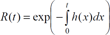
where R(t) is the reliability function or the survival function, and F(t) is the unreliability function.

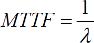
The most common measure of reliability provided by manufacturers is the mean time to failure (MTTF). MTTF is the expected value of the reliability:

$$MTTF=\underset{0}{\overset{\mathrm{\infty }}{\int }}R(t)dt$$

(2)

The hazard rate h(t) is the instantaneous rate of failure at a given time. The reliability function and the hazard rate are related as

$$R(t)=\text{exp}(-\underset{0}{\overset{t}{\int }}h(x)dx)$$

(3)

3.2 Reliability model

Reliability models are descriptions of how the hazard rate changes over time. For many electronic and mechanical devices, when the hazard rate is plotted as a function of time, the resulting curve resembles Fig. 1. This characteristic shape is referred to as the bathtub curve.

Fig. 1.

The bathtub curve

The bathtub curve has three distinct regions. At the left side of the curve, the hazard rate decreases with time. This corresponds to the period during which items fail largely due to defects in materials or construction. There are many early failures, but as defective items drop out of the population, the remaining population has a lower hazard rate. This is referred to as the burn-in or infant mortality period.

In the middle section, there is a period of approximately constant hazard rate, where random failures dominate. This period is referred to as the service life or useful life. At the right side, the hazard rate increases with time. During this period, components have reached the end of their useful lives and begin to fail due to deterioration. This is referred to as the wearout phase

3.3 Application to mobile robots

In our reliability model we consider robots to be made of multiple independent modules. We use module here to refer to some subsystem of interest. While we have a particular concept of module in mind for our research purposes, the reliability model proposed here is not tied to our specific module concept. The modules could, for instance, be functional divisions of the robot as in Fig. 2, or they could simply be all the individual components making up the robot.

Fig. 2.

Modular robot concept

In applying the bathtub model to robot modules, we assume that there will be a period of initial testing which allows burn-in failures to be dealt with before components are placed into service.

We also assume that the service life of components will be specified by the manufacturers and observed in mission planning so that modules will be removed from service before wearout failures begin to dominate.

Given these two assumptions, the hazard rate of a robot module needs to be known only during the service life phase. This hazard rate is modeled as a constant and can therefore be defined by a single value. Since it is also important to know when this hazard rate is valid, a second value is needed to indicate when the end of the service life is reached. The reliability of a module can therefore be modeled with just two parameters—the (constant) hazard rate and the service life length.

3.4 Consequences of constant hazard rate

A constant hazard rate is represented in the literature by λ. Substituting into (3) gives

$$R(t)=e^{-\lambda t}$$

(4)

Thus, the reliability of a device with a constant hazard rate is equal to one at the beginning of the service life and decays exponentially towards zero.

Substituting (4) into (2) yields the MTTF:

$$MTTF=\frac{1}{\lambda }$$

(5)

The relationships in (4) and (5) allow us to calculate the probability of failure of a component from the manufacturer's published MTTF. It is important to remember that this MTTF applies only during the central, constant-hazard-rate portion of the bathtub curve. It is a common mistake to assume that MTTF measures how long an item will last (Wilkins, 2002). For most components, the MTTF is much greater than the service life, so the item will fail due to wearout long before the time corresponding to MTTF is reached.

3.5 Combining reliabilities

The preceding information allows us to evaluate the reliability of a single module. We also need to be able to combine module reliabilities in order to evaluate the reliability of entire robots. In the examples in this paper, components are combined in series to build modules, and modules in series to build robots. For modules in series, the system is operational only when each module is operational. Therefore, the reliability of a system with N modules in series can be expressed as

$$R_S=\prod _{i=1}^N{R}_i$$

(6)

When each module has a constant hazard rate, the system hazard rate is

$${\lambda }_s=\sum _{i=1}^N{\lambda }_i$$

(7)

4. Application to Mission Design

4.1 Single-task reliability

We now apply the formulas described in the preceding section to predict the probability that a robot will complete a mission task. Consider a planetary exploration robot that is tasked to extract core samples. The robot is composed of five modules: power, computation and sensing, mobility, communications, and manipulator. The duration of the task is eight hours, and the amount of time each module is used during the task is listed in Table 1.

Table 1.

Module usage during sampling task

Module	Usage (h)
Power	8
Computation & Sensing	8
Mobility	6
Communications	2
Manipulator	4

For each module, we obtained reliability data representative of components used in NASA's planetary robots. The breakdown of components and reliabilities for the power module is shown in Table 2 as an example.

Table 2.

Components comprising power subsystem

Component	Quantity	MTTF (h)
Battery	2	4.8M
Battery control board	2	2.5M
Mission clock	1	10M
Power distribution unit	1	588k
Power control unit	1	5.3M
Shunt limiter	1	88k
Electrical heater	2	333k
Radioisotope heater	2	73k
Thermal switch	2	11k

These component reliabilities were combined for each module according to (7), giving the module MTTFs listed in Table 3.

Table 3.

Robot subsystem reliabilities

Module	MTTF (h)
Power	4202
Computation & Sensing	4769
Mobility	19724
Communications	11876
Manipulator	13793

Using the overall module failure rates and Eq. (4), we can calculate the probability that each module will still be functioning at the end of the task. For the power module this gives

$$R=\text{exp}(-8/4202)=99.810\mathrm{\%}$$

The reliabilities for the other modules for this task are found similarly and are shown in Table 4.

Table 4.

Module reliabilities during sampling task

Module	Task Reliability
Power	99.810%
Computation & Sensing	99.832%
Mobility	99.970%
Communications	99.983%
Manipulator	99.971%

Finally, we combine all of the module reliabilities using Eq. (6) to give an overall probability of task completion (POTC) of 99.567%.

4.2 Mission reliability

In order to determine the reliability of an entire mission, we break the mission into tasks, and for each task calculate the probability that the robot(s) will survive that task. In our analyses, we assume that failure occurs only at the end of a task. This allows us to avoid dealing with partially completed tasks. This simplification does not limit the resolution of the representation because tasks can be restated into smaller subtasks if needed.

4.2.1 Analytical method

For very simple missions, it is possible to enumerate by hand all of the possible task outcomes. One way of doing this is by drawing a tree diagram such as in Fig. 3. We can use the tree to derive an analytical solution for the probability of mission success. For the two-task, two-robot mission shown in Fig. 3, this analytical solution would simply be

$$P(s)=P(T1{)}^2\cdot P(T2{)}^2$$

(8)

Fig. 3.

Tree for two-task, two-robot mission

where P(T1) and P(T2) are the probabilities of a single robot surviving each of the tasks. (In Fig. 3 we use the shorthand R1⁺ and R1⁻ to represent that robot 1 is alive or dead, respectively.)

For more complex missions, it can be difficult to enumerate the possible outcomes by hand. The size of the tree grows rapidly in the number of robots, the number of tasks, and for repairable robots, the number of spare parts. As an example, we show in Fig. 4 the same mission as Fig. 3, but with the addition of a spare module. By adding a single spare module, the number of leaf nodes has increased from 7 to 25. For a realistic scenario with several robots, multiple tasks and perhaps dozens of spare parts, the tree becomes complex enough that hand calculation is infeasible.

Fig. 4.

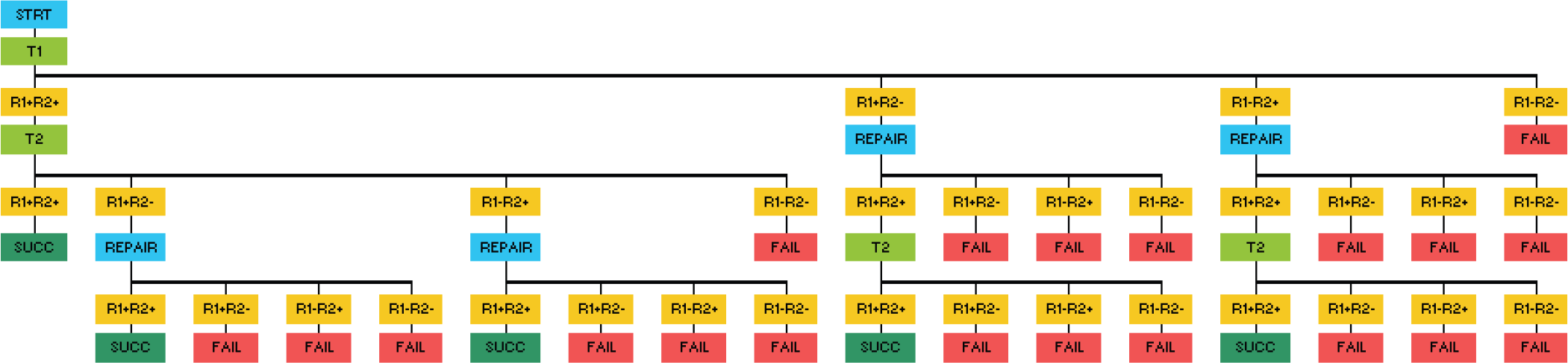
Probability tree for two-task, two-robot mission with one spare module

4.2.2 Stochastic method

In order to calculate the reliability of complex missions without a great deal of tedious and error-prone hand derivations, we have developed a more automated method for solving these problems using stochastic simulation.

In this method, we represent the mission using a state-transition diagram. A simplified diagram for a generic two-task mission is shown in Fig. 5. We then implement the state machines represented by these diagrams in software.

Fig. 5.

State transition diagram for two-task mission

The state of each robot (alive or dead) is evaluated at each task node by choosing a random value between 0 and 1 for each module and comparing that value with the probability of survival for that module for that task. The branch in the diagram corresponding to the resulting team state is followed, and the process continues until the system reaches either Success or Failure.

As an example, if Task 1 in Fig. 5 corresponds to the sampling task discussed in section 4.1, then after Task 1 we would “roll the dice” for each module on each robot and compare the values with those in Table 4. If all the modules survived this task, then we continue on the main branch of the diagram to Task 2. If one or more modules failed, then if there are spares (robots or modules) available, then a repair action is performed ¹ . If there are no spares available, then the mission fails.

The simulation is repeated many times, with each Success result being assigned a score of one and each Failure result being assigned a score of zero. The average score of all trials then gives the overall probability of mission completion (PoMC).

5. Results for Sample Mission with Repairable Robots

5.1 Mission and tasks

For this analysis, we consider a simple robotic mission to install a solar panel array for a measurement and observation outpost. The installation task consists of carrying the panels from the drop zone to the outpost and then assembling them. The size of the panels is such that two robots are needed to carry and assemble one panel.

For the purposes of the reliability analysis, the task of assembling a solar panel is broken down into three subtasks:

–

Transit to the outpost

–

Assemble the panel

–

Return to the drop zone

Repairable robots have the additional subtask Repair. The usages of each module for each subtask are shown in Table 5. These usage times were assigned using reasonable assumptions about the relative durations of different tasks and the relative usage of different modules. The usage for the Return task is considered to be the same as for the Transit task.

Table 5.

Module usage by task, in hours.

Module	Transit	Assemble	Repair
Power	6	8	4
Computation & Sensing	6	8	4
Mobility	6	4	2
Communications	2	4	2
Manipulator	0	8	4

5.2 Robot teams

Our baseline robot team consists of a pair of robots that are constructed to very high levels of robustness. These robots are composed of highly reliable components, are designed with operating limits well beyond the expected operating conditions, and incorporate redundancy and self-diagnostic capabilities. We use the MTTF values listed in Table 1 for this robot team, since the component failure rates used to derive these values are representative of current NASA robots.

Against this baseline configuration, we consider alternative team configurations employing redundancy (additional robots) and self-repairability (additional parts).

5.3 Repair

Spares (either robots or modules) are stored at the drop zone. For the repairable team, when a failure occurs, the robot executing the repair must first retrieve a spare module from the drop zone and then return to the failed robot to execute the repair.

Because we consider failure only at the ends of tasks, robots will always fail either at the drop zone or at the outpost. There are therefore two different repair actions to be considered for the repairable team. If a failure occurs at the outpost, the robot executing the repair must transit to the drop zone, retrieve a spare module, return to the outpost, and then execute the repair. If the failure occurs at the drop zone, then the robot needs only to pick up a spare module and execute the repair.

For the nonrepairable team, the “repair” action (a new robot replacing the failed one) is also different depending on the location of the failure and which task was most recently completed. With one spare robot, there are two possible repair actions. If a single robot fails after the transit task, then the replacement robot will need to transit to the outpost to perform the assembly task. If a single robot fails after the assembly task, then the replacement robot will wait at the drop zone for the surviving robot to return.

5.4 Input variables

For this mission scenario, once the tasks and the task durations are fixed, then the input variables in our model are:

–

the number of spare robots

–

the number of spare modules of each type

–

the reliability of the components used, and

–

the mission duration (number of panels to install)

5.5 Design questions

Given these variables, there are a number of questions that a mission designer might ask. For example:

“For a given mission duration and component reliability, what is the fewest number of spare robots (or spare parts) required to meet a certain probability of mission completion?”

and

“If additional spares are added beyond the minimum number, can we use lower reliability components and, if so, how much lower?”

5.5.1 Minimum number of spares required

Our initial comparison is of teams using different numbers of spare robots or spare modules. Fig. 6 shows the simulation results for teams with zero to two spare robots (2NR = two non-repairable robots, etc.), and teams with one to five spare modules (2RR+1 = two repairable robots with one spare module, etc.).

Fig. 6.

Varying numbers of spares with same module reliabilities

For the repairable robot teams the spare modules are assigned according to the reliability of the modules, i.e., the team with one spare module has one spare of the lowest-reliability module (the power module), the team with two has one of each of the two lowest-reliability modules (power and computation/sensing), etc.

Using Fig. 6, a mission designer can immediately eliminate team configurations that do not deliver high enough reliability. For instance, if the intended mission duration is 20 panels, and the minimum acceptable PoMC is 80%, Fig. 6 indicates that at least two spare modules or one spare robot is needed to meet these requirements.

5.5.2 Minimum MTTF with spares

Fig. 7 compares a single repairable team configuration (2RR+3) using different component reliabilities. Such a comparison allows us to determine the minimum component reliability which will provide a required PoMC for a particular team configuration.

Fig. 7.

Constant team configuration (2RR+3) with varied component reliabilities

Each team in Fig. 7 has three spare modules (one spare for each of the three lowest-reliability subsystems). When varying the reliability of the components, we apply a constant multiplier to all of the MTTF values in Table 3. For instance, when we refer to a team with 20% of the MTTF of the baseline team, we are multiplying all the values in Table 1 by 20%.

For the hypothetical mission requirement of 20 panels and 80% probability of success, Fig. 7 indicates the ability to build the 3-spare-module team using components having 60% of the baseline reliability.

5.5.3 Cost

Probability of mission completion is not the only factor to consider when choosing among robot team configurations

Another important consideration is cost. Redundancy and repairability allow us to achieve a given level of mission reliability using lower-reliability components. We would like to know if this can reduce the overall mission cost.

We can compare the cost of the robots themselves by hypothesizing a one-to-one relationship between component reliability and cost. With this assumption, a team of four robots where each robot has 50% of the reliability of the baseline robots should cost the same as the two-robot baseline team. Similarly, we should be able to acquire four spare modules with 50% of the baseline reliability for the same cost as two with the baseline reliability. ²

Using this cost-reliability hypothesis we can configure teams with different numbers of spare modules to have equal cost. In order to avoid the need to hypothesize about the relative costs of the different modules, we have compared teams with multiples of complete sets of modules, i.e., 5, 10, and 15 modules. Fig. 8 shows a comparison of these configurations.

Fig. 8.

Teams with equal component cost

Fig. 8 clearly shows that for a fixed component cost, it is much better to use lower reliability components and have spares than to use higher reliability components without spares. Fig. 8 also shows that there are diminishing returns as the number of spares is increased (when keeping total component cost constant). Since other costs (such as logistics and transportation) will increase with the number of spare modules, there is probably an optimal number of spare modules for this mission, given a fixed component cost and the incremental cost per module for transportation, logistics, etc.

5.5.4 Time

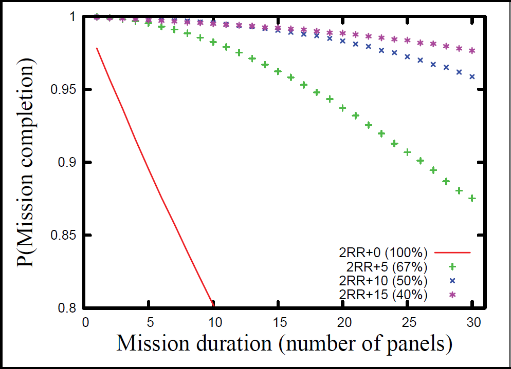
We expect that repairable teams with lower-reliability components will spend a greater amount of time repairing each other instead of working on their primary mission tasks. If a mission must be completed quickly, then it may be advantageous to use higher-reliability components. Fig. 9 compares the same teams as Fig. 8 on the basis of average time elapsed per completed panel.

Fig. 9.

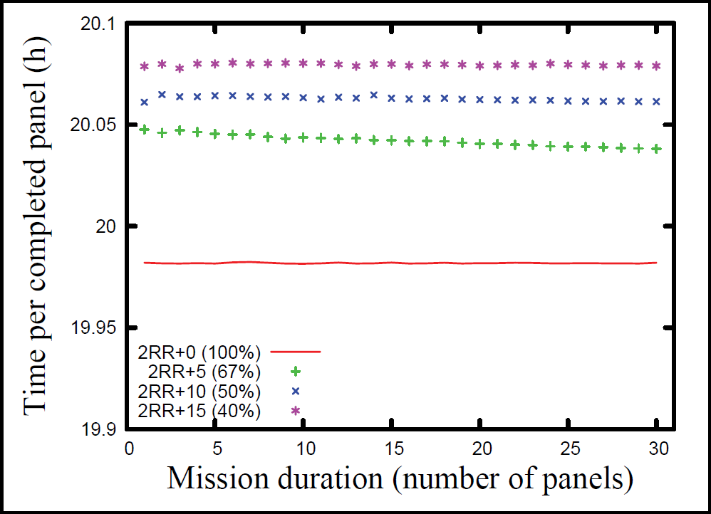
Average time required per completed panel

Fig. 9 shows that there is indeed a time penalty for the repairable teams, but the difference between the teams is very small. The worst-performing team requires about 0.5% more time per panel than the baseline team.

5.5.5 Spare robots versus spare modules

When considering options for improving PoMC or reducing cost, a mission designer might want to know whether it is better to use nonrepairable robots with spare robots or repairable robots with spare modules. One way to determine this is to compare two teams with similar cost and see which has the higher PoMC.

A team with a set of five spare modules, one of each type, should have component costs similar to those of a team with one spare robot. Transportation and other logistics costs should be similar for the two teams, since they have similar mass and volume. Given this equality of cost, we would like to determine which option would provide higher reliability.

Fig. 10 shows the simulation results for a three-robot team and a repairable team, each having 60% of the baseline reliability. The repairable team has a complete set of five spare modules. Fig. 10 shows that spare parts are a much better choice for this mission than spare robots. For instance, for a mission duration of 25 panels, the team with spare modules has a mission reliability of about 89% vs. about 77% for the team with a spare robot.

Fig. 10.

Spare robots vs. spare modules

We also see from Fig. 10 that the team with five spare modules and 60% reliability provides approximately the same mission reliability as the team with three robots and 100% reliability. In other words, the repairable team can provide the same mission reliability at 40% lower cost.

6. Discussion

6.1 Limitations

In its current form, the methodology described in this paper has limited applicability. Some of the reasons for this are given below.

6.1.1 Types of failure addressed

As mentioned in section 2, most mobile robots today do not fail due to the types of hardware failure which are modeled by reliability engineering. Among current robots, NASA's planetary robots, military UAVs, and perhaps some consumer robots are designed and built to high enough standards that these methods can be applied meaningfully. However, the number of robots for which reliability engineering can provide meaningful predictions should increase significantly as robots enter the mainstream and begin to be built by companies with experience in manufacturing reliable complex machines.

6.1.2 Availability of reliability data

With current robot design methods, reliability specifications for components are rarely considered. In order for our methods to be applied, it will be necessary to choose components which have a known MTTF, or else to perform in-house testing in order to determine component reliabilities. This is again something which we expect to happen as robots become more prevalent.

6.1.3 Acceptable failure rates

If our methodology is to be used as a design tool which can take a set of mission requirements and provide a configuration or configurations that meet the requirements, then it is necessary for a mission designer to specify the acceptable probability of mission failure.

Our experience has been that most roboticists do not have an answer when asked “How much failure is acceptable?” Also, in many cases the meaning of the PoMC is not intuitive. In the case of a consumer product the difference between 80% PoMC and 90% PoMC is fairly easy to grasp-we can expect 20% vs. 10% of customers to be unhappy due to product failure. But in the case of a one-off robot team for planetary exploration, what is the consequence of 20% vs. 10% chance of failure?

While the latter question is beyond the scope of this work, we can suggest one way to find an answer: If we can provide costs for different robot team configurations, and a reward value for completing the mission, then we can calculate the expected value for each team based on those dollar values and its PoMC. The preferred team would then be the one which maximizes the expected value.

6.1.4 Operating conditions

One aspect of published component failure rates which is often overlooked is that they are valid only under a given set of environmental and operating conditions. For many components the failure rate is affected by environmental conditions, such as temperature, as well as operating conditions, such as speed. For many applications, the range of operating conditions may be small enough that we can ignore these factors. However, some applications, such as planetary rovers, have extreme ranges of operating conditions which will have a significant effect on the PoMC.

As an example, a rule of thumb for the effect of temperature on many components is that the MTTF is halved for every 10°C rise in temperature. Mars rovers experience temperature differences of 60°C between day and night, which implies a 64-fold change in reliability for some components. Accurate prediction of robot team reliability in such extremes will require incorporation of models for the effects of environmental and operating conditions.

6.1.5 Mission specification

While the stochastic method described in section 4.2.2 is much more user-friendly than the analytic method described in 4.2.1, there is still a significant amount of work involved in programming the state diagram for a mission specification. In order for this methodology to become usable by a mission designer it will be necessary to implement some method of taking a mission specification and automatically generating a machine representation which can be used for the simulation. While we have not yet investigated avenues for accomplishing this, we expect that this is a problem which has been encountered by most mission planning software and that we should therefore be able to borrow a pre-existing solution to this problem.

6.2 Other considerations

In addition to providing tools which a mission designer can use to evaluate a specific mission, we would also like to examine a large number of varied missions in order to determine if generalizations can be made about classes of missions. Perhaps there are some classes of robotic missions for which repairability is always better than spare robots, and other classes for which the opposite holds. Our hope is that we can identify patterns which will provide rules of thumb which a mission designer can use in order to identify appropriate team configurations for a mission.

7. Summary

We have shown in this paper how reliability can be used as a design tool for multirobot missions. The method presented here is the first principled quantitative method for performing mission reliability estimation for mobile robot teams.

We applied this method to an example robot mission, examining the cost-reliability tradeoffs among different team configurations. In particular we examined teams using either redundancy (spare robots) or repairability (spare components). Using conservative estimates of the cost-reliability relationship, our results show that it is possible to significantly reduce the cost of a robotic mission by using cheaper, lower-reliability components and providing spares.

Our results suggest that the current design paradigm of building a minimal number of highly robust robots may not be the best way to design robots for extended missions.